

Background
In this tutorial we demonstrate the use of StarBEAST2, a fully Bayesian method of species tree estimation and a replacement for BEAST (Heled & Drummond, 2010). StarBEAST2 is many times faster than BEAST, and also supports applying a relaxed clock to the species tree. This enables estimating the substitution rates of extant and ancestral species under a multispecies coalescent model.
You will need to download and install the following software:
Programs used in this Exercise
BEAST2 - Bayesian Evolutionary Analysis Sampling Trees 2
BEAST2 (http://www.beast2.org) is a free software package for Bayesian evolutionary analysis of molecular sequences using MCMC and strictly oriented toward inference using rooted, time-measured phylogenetic trees. This tutorial is written for BEAST v2.5 (Drummond & Bouckaert, 2014).
BEAUti2 - Bayesian Evolutionary Analysis Utility
BEAUti2 is a graphical user interface tool for generating BEAST2 XML configuration files.
Both BEAST2 and BEAUti2 are Java programs, which means that the exact same code runs on all platforms. For us it simply means that the interface will be the same on all platforms. The screenshots used in this tutorial are taken on a Mac OS X computer; however, both programs will have the same layout and functionality on both Windows and Linux. BEAUti2 is provided as a part of the BEAST2 package so you do not need to install it separately.
TreeAnnotator
TreeAnnotator is used to summarise the posterior sample of trees to produce a maximum clade credibility tree. It can also be used to summarise and visualise the posterior estimates of other tree parameters (e.g. node height).
TreeAnnotator is provided as a part of the BEAST2 package so you do not need to install it separately.
Tracer
Tracer (http://tree.bio.ed.ac.uk/software/tracer) is used to summarise the posterior estimates of the various parameters sampled by the Markov Chain. This program can be used for visual inspection and to assess convergence. It helps to quickly view median estimates and 95% highest posterior density intervals of the parameters, and calculates the effective sample sizes (ESS) of parameters. It can also be used to investigate potential parameter correlations. We will be using Tracer v.
FigTree
FigTree (http://tree.bio.ed.ac.uk/software/figtree) is a program for viewing trees and producing publication-quality figures. It can interpret the node-annotations created on the summary trees by TreeAnnotator, allowing the user to display node-based statistics (e.g. posterior probabilities). We will be using FigTree v.
Practical: Setting up the StarBeast2 analysis
This tutorial will guide you through the analysis of seven loci sampled from 26 individuals representing eight species of pocket gophers, a data set which was originally gathered and analysed by (Belfiore et al., 2008). The objective of this tutorial is to estimate the species tree that is most probable given the multi-individual multi-locus sequence data. The species tree has eight taxa, whereas each gene tree has 26 taxa. StarBEAST2 will co-estimate seven gene trees embedded in a shared species tree (Heled & Drummond, 2010).
The first step will be to convert a NEXUS file with a DATA or CHARACTERS block into a BEAST XML input file. This is done using the program BEAUti (Bayesian Evolutionary Analysis Utility). This is a user-friendly program for setting the evolutionary model and options for the MCMC analysis. The second step is to actually run BEAST using the input file that contains the data, model and settings. The final step is to explore the output of BEAST in order to diagnose problems and to summarize the results.
Setting up an analysis in BEAUti
Run BEAUti by double clicking on its icon, or by launching the BEAUTi executable file from the command line in Linux.
Set up BEAUti for StarBEAST2
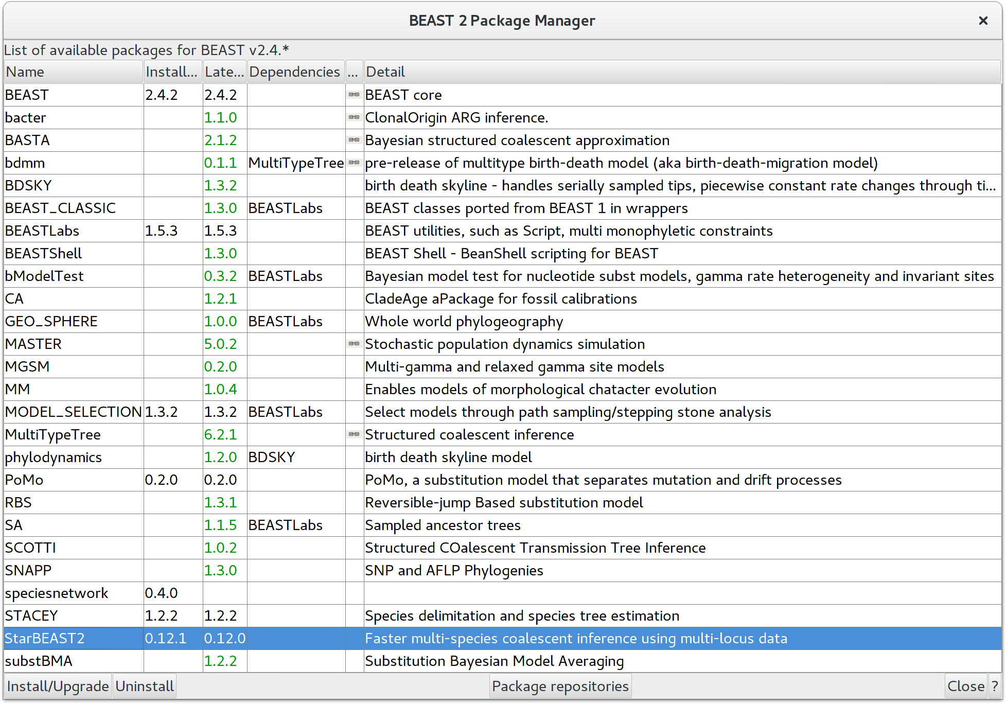
StarBEAST2 can be easily installed from within BEAUTi. First choose the
File/Manage Packages menu item, which will then display the list of
packages available for installation. Select
the StarBEAST2 package and then install it by clicking the
Install/Upgrade button. You must restart BEAUTi after installing any new
packages for new features to become available.
StarBEAST2 includes a series of templates for multispecies coalescent analyses. These include the StarBeast2 template for strict clock or gene tree relaxed clock analyses, and various SpeciesTree\ldots templates for species tree relaxed clock analyses. Currently three types of relaxed clocks are supported by StarBEAST2; the uncorrelated lognormal clock (UCLN), the uncorrelated exponential clock (UCED), and the random local clock (RLC) which we will use for this tutorial. The first thing to do is selecting that template by choosing the File/Template/SpeciesTreeRLC menu item. When changing a template, BEAUti deletes all previously imported data and starts with a new empty template. So, if you already loaded some data, a warning message pops up indicating that this data will be lost if you switch templates.

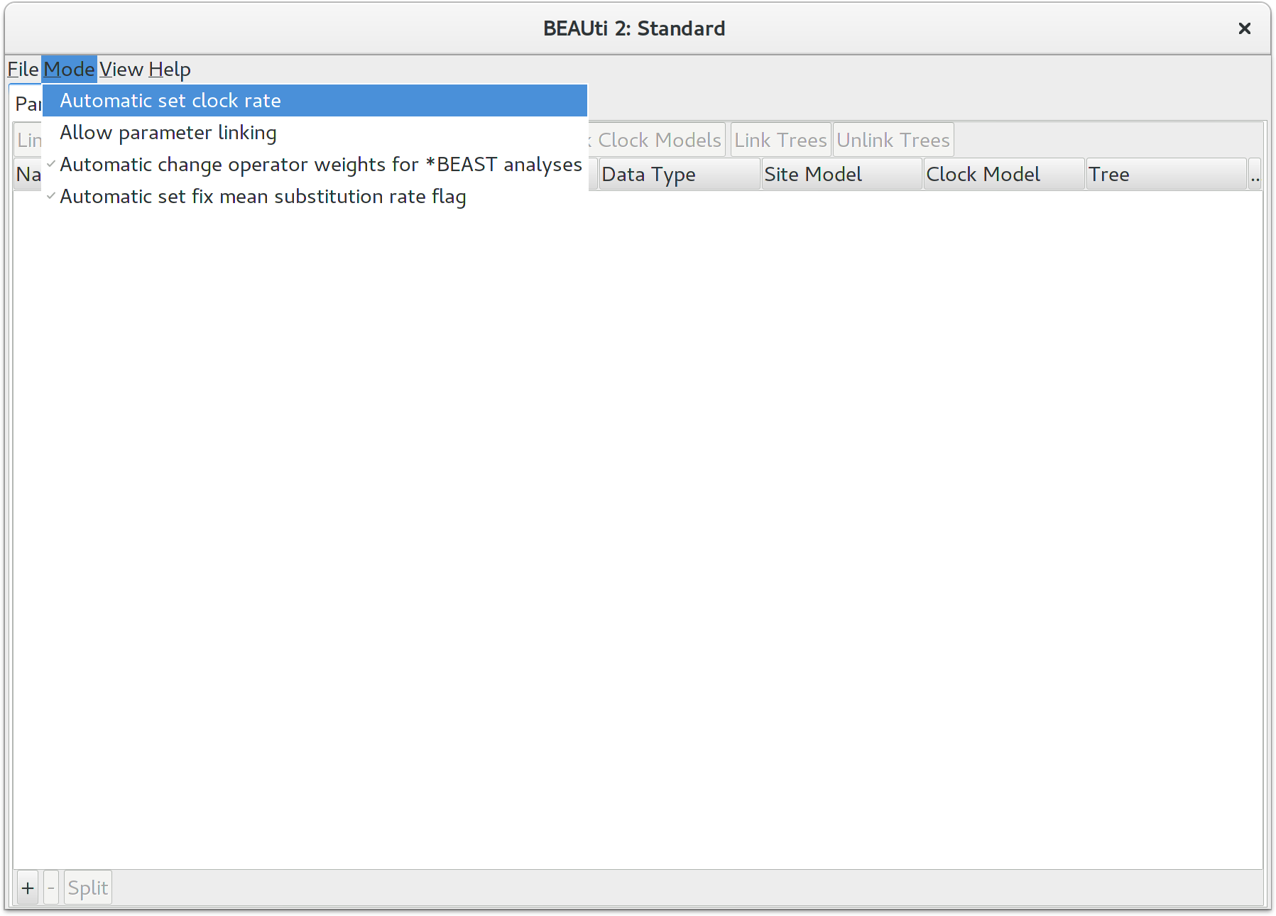
Allow clock rates to vary
By default BEAUTi fixes the clock rate of the first partition to 1, so that
the rates of other loci are estimated relative to the first locus. This is
generally inappropriate for StarBEAST2 analyses, so it is very
important to disable this behaviour by deselecting the Mode/Automatic
set clock rate menu item.
Loading the NEXUS files
StarBEAST2 supports multiple individuals per-species and multiple loci (we use the term locus to refer to a genomic sequence, and gene when referring to the evolutionary tree for a given locus). The data for each locus is stored as one alignment in its own NEXUS file. Taxa names in each alignment have to be unique, but duplicates across alignments are fine.
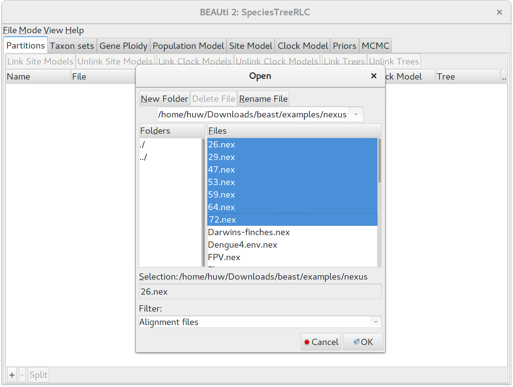
To load a NEXUS format alignment, click the button with the plus symbol (+) in the lower left corner of the main Partitions tab. For this tutorial, navigate to the examples/nexus subfolder inside the beast application folder, and select all of the first seven NEXUS files. They should be numbered 26, 29, 47, 53, 59, 64, and 72.
Once loaded, the imported alignments are displayed in the \textbf{Partitions} panel. You can double click any alignment (partition) to show its detail. For multi-locus analyses, BEAST can link or unlink substitutions models across the loci by clicking buttons on the top of the panel. The default of StarBEAST2 is to unlink all models: substitution, clock, and trees. Note that you should only unlink the tree model across data partitions that are actually genetically unlinked. For example, in most organisms all the mitochondrial genes are effectively linked due to a lack of recombination and they should be set up to use the same tree model in any multispecies coalescent analysis.
Assigning the correct species to each sequence
Each taxon in a StarBEAST2 analysis is associated with a species or similar OTU. Typically the species name is already embedded inside the taxon label. The species name should be easy to extract; place it either at the beginning or the end, separated by a special character which does not appear in names. For example, aria_334259, coast_343436 (using an underscore) or 10x017b.wrussia, 2x305b.eastis (using a dot).
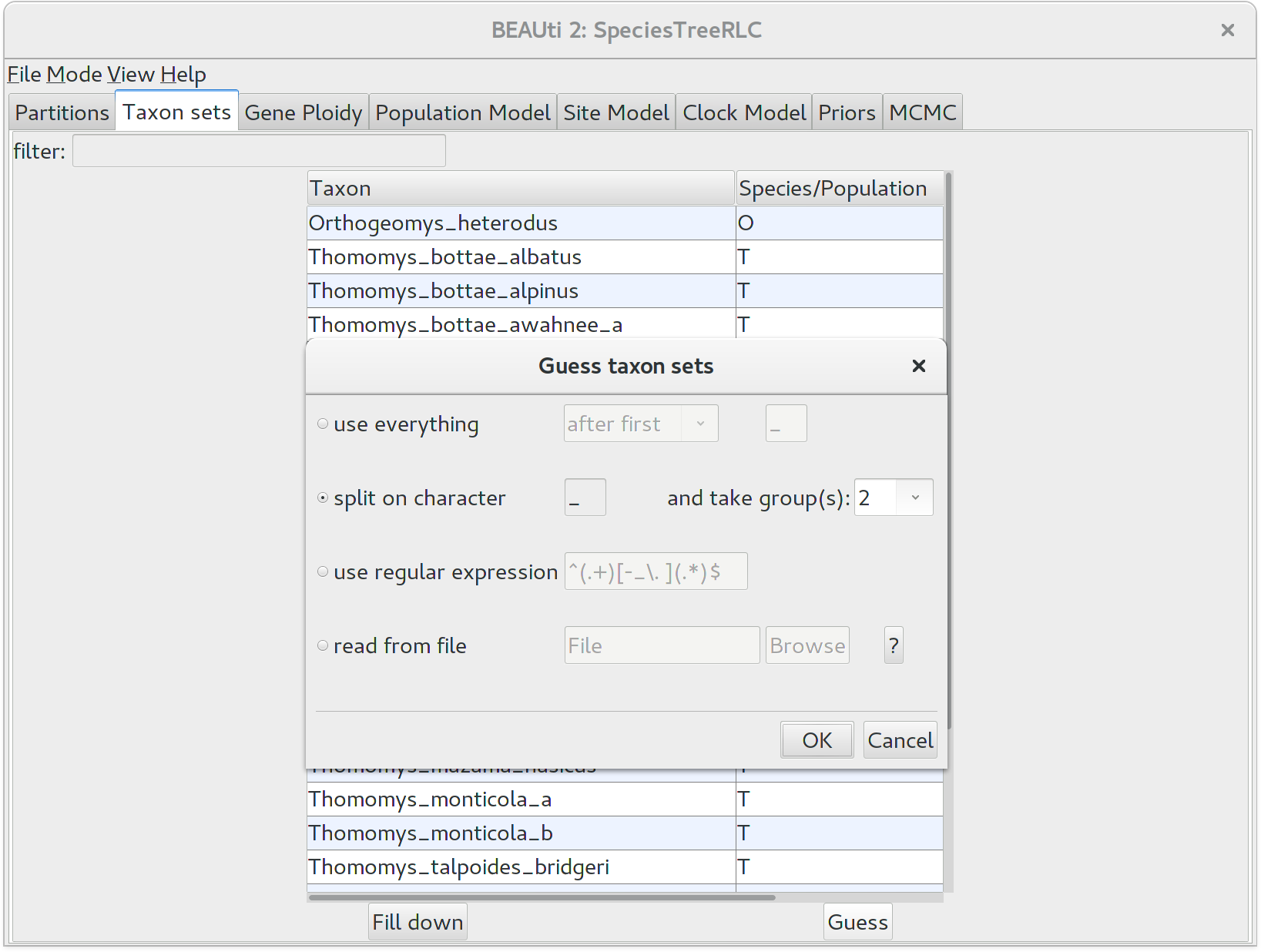
We need to tell BEAUti somehow which lineages in the alignments go with taxa in the species tree. Select the Taxon Set panel, and a list of taxa from the alignments is shown together with a default guess by BEAUti. In this case, the guess is not very good, so we want to change this. You can manually change each of the entries in the table, or press the guess button and a dialog is shown where you can choose from several ways to try to detect the taxon from the name of the lineages, or have a mapping stored in a file. In this case, splitting the name on the underscore character _ and selecting the second group will give us the mapping that we need.
Alternatively, the mapping can be read from a trait file. A proper trait file is tab delimited. The first row is always traits followed by the keyword species in the second column and separated by tab. The rest of the rows map each individual taxon name to a species name: the taxon name in the first column and species name in the second column separated by tab.
Adjusting the ploidy of each gene
Ploidy should be based on the mode of inheritance for each gene. By convention, nuclear genes in diploids are given a ploidy of 2.0. Because mitochondrial and Y chromosome genes are haploid even in otherwise diploid organisms, and also inherited only through the mother or the father respectively, their effective population size Ne is only one quarter that of nuclear genes. Therefore if nuclear gene ploidy is set to 2.0, mitochondrial or Y chromosome gene ploidy should be set to 0.5. In this analysis all genes are from nuclear loci and their ploidy should be left at the default value of 2.0.
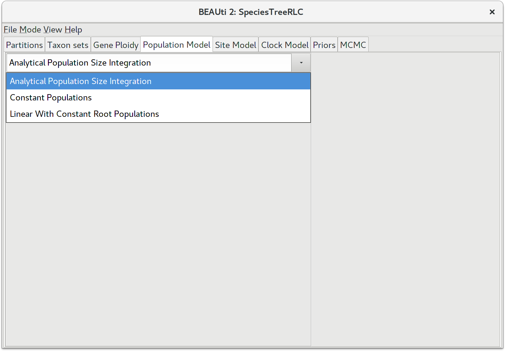
Selecting the method of population size integration
StarBEAST2, like BEAST before it, can estimate the effective population sizes for extant and ancestral species. However by default StarBEAST2 analytically integrates over population sizes which is faster than making explicit estimates. If you do need to estimate population sizes, change the population model to Constant Populations. For this tutorial, keep the default model which is Analytical Population Size Integration.
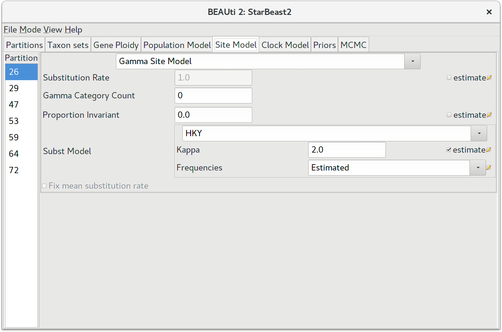
Setting the substitution model
The next thing to do is to click on the Site Model tab at the top of the main window. This will reveal the evolutionary model settings for BEAST. Exactly which options appear depend on whether the data are nucleotides, or amino acids, or binary data, or general data. The settings that will appear after loading the data set will be the default values so we need to make some changes.
Many of the models may be familiar to you. For this analysis, we will select each substitution model listed on the left side in turn to make the following change: select HKY for substitution model (Subst Model). Make sure to repeat this step for every partition listed on the left side.
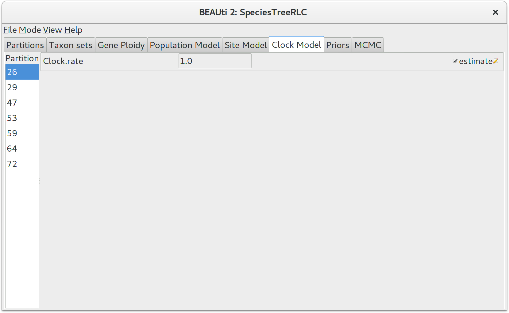
Setting the clock model
Click on the Clock Model tab at the top of the main window. In this panel you can configure the mean clock rate for each locus. If you followed the earlier instructions to disable automatic setting of clock rates, the mean clock rate Clock.rate of all partitions should have the estimate box ticked.
The default prior for mean clock rates in StarBEAST2 is a lognormal distribution with a mean (in real space) of 1. Trees estimated using this prior will have a time axis in units of substitutions. This will not be appropriate when using fossil (or other external) calibrations. You might instead use a 1/X prior, which is uninformative and will allow the calibration(s) to guide the clock rates.
Priors
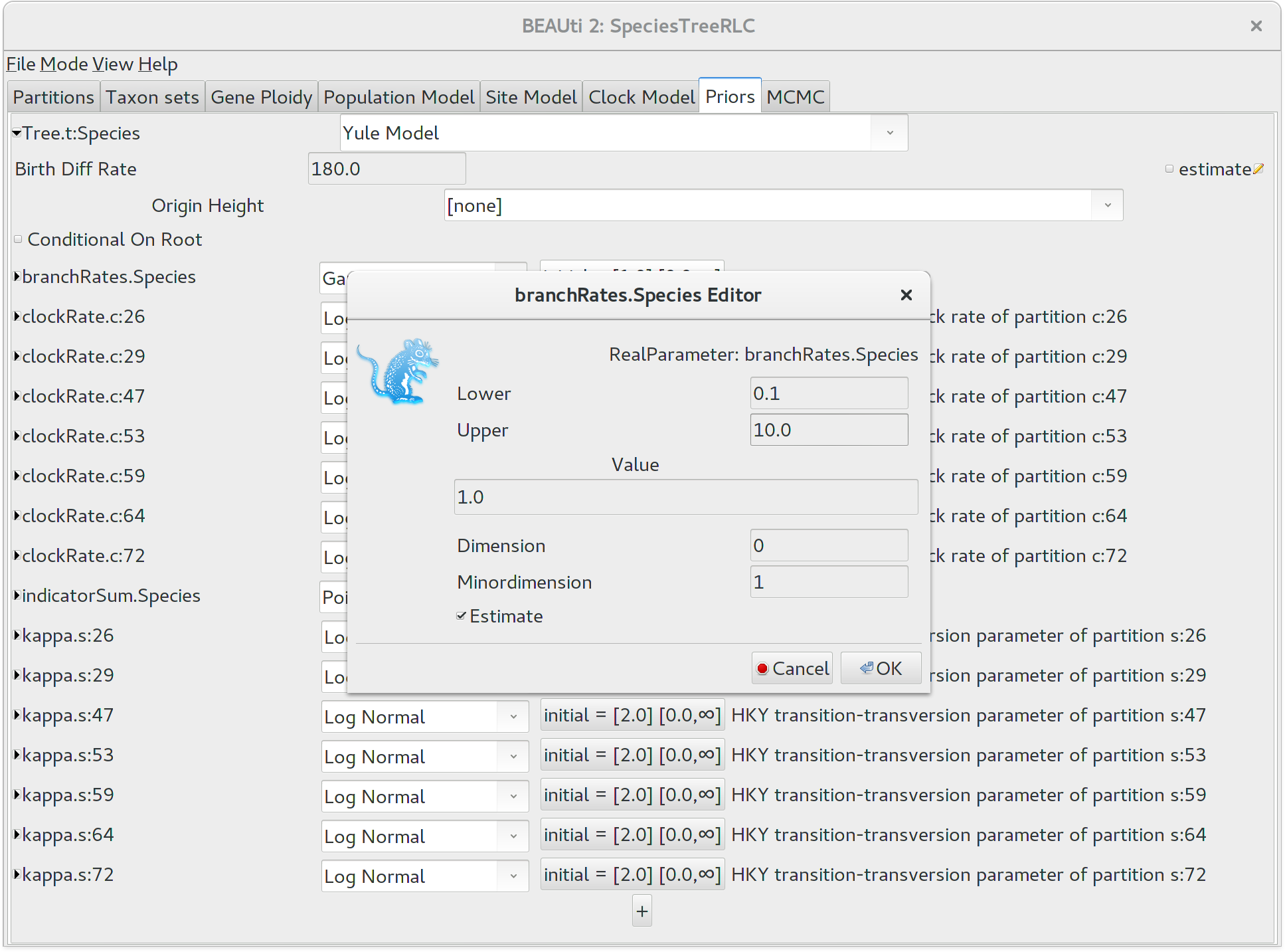
The Priors panel allows priors to be specified for each parameter in
the model. Click the top-leftmost arrow to expand the options available for the
default Yule Model, and set the speciation rate (called for some silly
historical reason Birth Diff Rate) to 180.0. Uncheck the
estimate box to make this a fixed parameter. For real
analyses you should almost certainly estimate this value, but a fixed value will
help us complete the tutorial in a reasonable time frame.
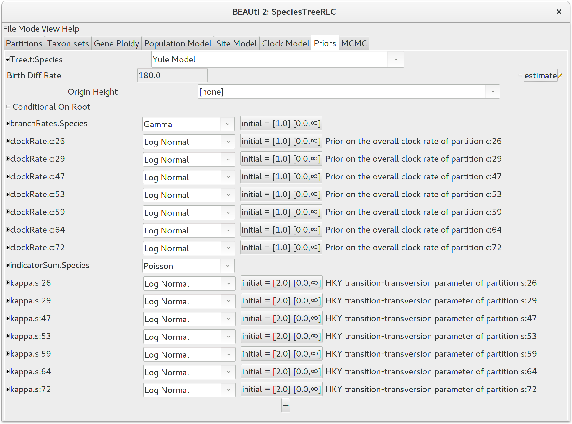
It would be biologically implausible for closely related species to have very large differences in substitution rates, so we should constrain the per-species branch rates to a reasonable range of values. Click the button next to branchRates.Species to define this range. Change Lower to 0.1 and Upper to 10.0, which means that the fastest branch rate can not be more than 100 times that of the slowest branch rate.
Setting the MCMC options
The next tab, MCMC, provides more general settings to control the length of the MCMC and the file names.
First up is the Chain Length. This the number of steps BEAST will complete before stopping an MCMC chain. The appropriate length of the chain depends on the size of the data set, the complexity of the model and on the accuracy of the answer required. The default value of 10,000,000 is entirely arbitrary and should be adjusted according to the size of your data set. For this tutorial keep the default chain length, which should finish within 10 to 20 minutes on a modern computer.
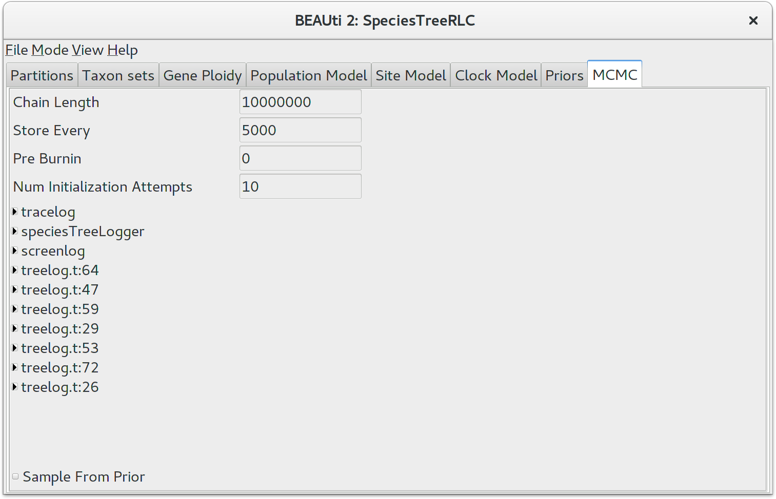
The other options specify how the parameter values in the Markov chain should be displayed on the screen and recorded in the log file. The screenlog output is simply for monitoring the programs progress so can be set to any value (although if set too small, the sheer quantity of information being displayed on the screen will actually slow the program down). For the tracelog and treelog files, the value should be set relative to the total length of the chain. Sampling too often will result in very large files with little extra benefit in terms of the precision of the analysis. Sample too infrequently and the log file will not contain much information about the distributions of the parameters. You probably want to aim to store no more than 10000 samples so this should be set to no less than (chain length)/10000. For this exercise, leave the default Store Every and Log Every settings in place.
If you are using Windows then we suggest you add the suffix .txt to the tracelog, speciesTreeLog, and other treelog file names (e.g. starbeast.log.txt and species.trees.txt) so that Windows recognizes them as text files.
Generating the BEAST XML file
We are now ready to create the BEAST XML file. To do this, either select the File/Save or File/Save~As menu options. Save the file with an appropriate name (we usually end the filename with .xml, e.g. pocket-gophers-rlc.xml). We are now ready to run the file through BEAST.
Running BEAST
Now run BEAST and when it asks for an input file, provide your newly created XML file as input by clicking Choose~File…, and then click Run. In Linux BEAST will immediately launch a file opening dialog box, which is to select the BEAST XML to run. BEAST will then run until it has finished reporting information to the screen. The actual results files are saved to the disk in the same location as your input file.
Analyzing the results
Run the program called Tracer to analyze the output of BEAST. When the main window has opened, choose Import Trace File… from the File menu and select the file that BEAST has created called starbeast.log. On the left hand side is a list of the different quantities that BEAST has logged. There are traces for the the various probabilities and likelihoods as well as estimates of various discrete and continuous parameters. The first and most important trace — the posterior — is the log of the product of gene tree phylogenetic likelihoods, the coalescent probability of gene trees within the species tree, and all prior probabilities. Selecting a trace on the left brings up analyses for this trace on the right hand side depending on tab that is selected. Select the statistic named sum(indicators.Species) — this is the total number of substitution rate changes along the species tree. You should now see a window like below.
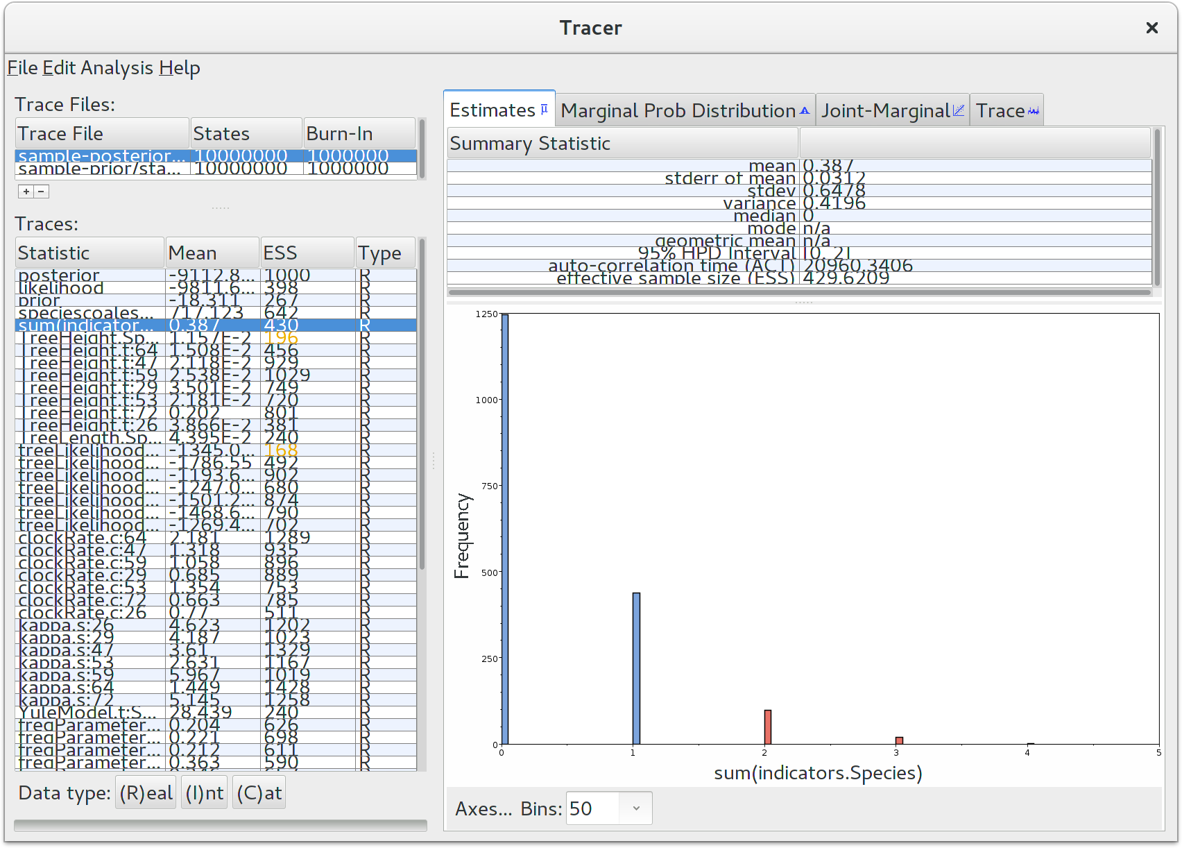
Remember that MCMC is a stochastic algorithm so the actual numbers will not be exactly the same. Tracer will plot a (marginalized) posterior distribution for the selected parameter and also give you statistics such as the mean and median. The 95\% HPD interval stands for highest posterior density interval, and represents the most compact interval on the selected parameter that contains 95% of the posterior probability. It is also known as a credibility interval, and can be thought of as a Bayesian analog to a confidence interval. The HPD for the sum of rate changes suggests that either 0, 1 or 2 rate changes have occured.
A note on prior distributions
For any Bayesian analysis, it is very important to compare your findings with the prior distribution. The default prior distribution for the number of substitution rate shifts for a random local clock is a Poisson distribution with the \lambda parameter fixed at ln(2), which is approximately 0.69. The prior probability of zero rate changes for the default distribution is equal to 50%. Tracer reported that around 1250 samples had zero rate shifts (out of 9000000/5000 = 1800) post-burnin posterior samples. This means that after adding data, our belief in a strict clock increased from 50% to about 70%, a very modest change. The data in this tutorial suggests that a strict clock applies to pocket gophers, but falls far short of any standard of proof.
Obtaining an estimate of the phylogenetic tree
BEAST also produces a sample of plausible trees. These can be summarized using the program TreeAnnotator. This will take the set of trees and identify a single tree that best represents the posterior distribution. It will then annotate this selected tree topology with the mean ages of all the nodes as well as the 95% HPD interval of divergence times for each clade in the selected tree. It will also calculate the posterior clade probability for each node. Run the TreeAnnotator program and set it up to look like in the figure below.
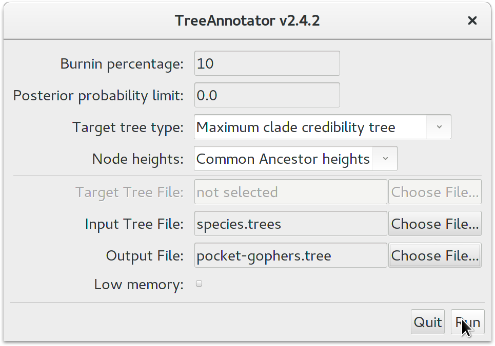
The Burnin percentage is the proportion of trees to remove from the start of the sample; for this tutorial, set a 10% burnin.
The Posterior probability limit option specifies a limit such that if a node is found at less than this frequency in the sample of trees (i.e., has a posterior probability less than this limit), it will not be annotated.
For Target tree type you can either choose a specific tree from a file or ask TreeAnnotator to find a tree in your sample. The default option, Maximum clade credibility tree, finds the tree with the highest product of the posterior probability of all its nodes.
Keep Common Ancestor heights for Node heights. This sets the heights (ages) of each node in the tree to the mean height of the most recent common ancestor across the entire set of trees in the posterior.
For the input file, select the trees file that BEAST created (by default this will be called species.trees) and select a file for the output (here we have called it pocket-gophers.tree). Now press Run and wait for the program to finish.
Viewing the species tree(s)
Finally, we can look at the tree in another program called FigTree. Run this program, and open the pocket-gophers.tree file by using the Open command in the File menu. The tree should appear. You can now try selecting some of the options in the control panel on the left. Try selecting Node Bars to get node age error bars. Turn on Node Labels and select posterior to get it to display the posterior probability for each node, and also turn on Branch Labels and select rate_95%_HPD to display the 95% HPD of the relative substitution rate for each species tree branch. You should end up with something like in the Figure below.
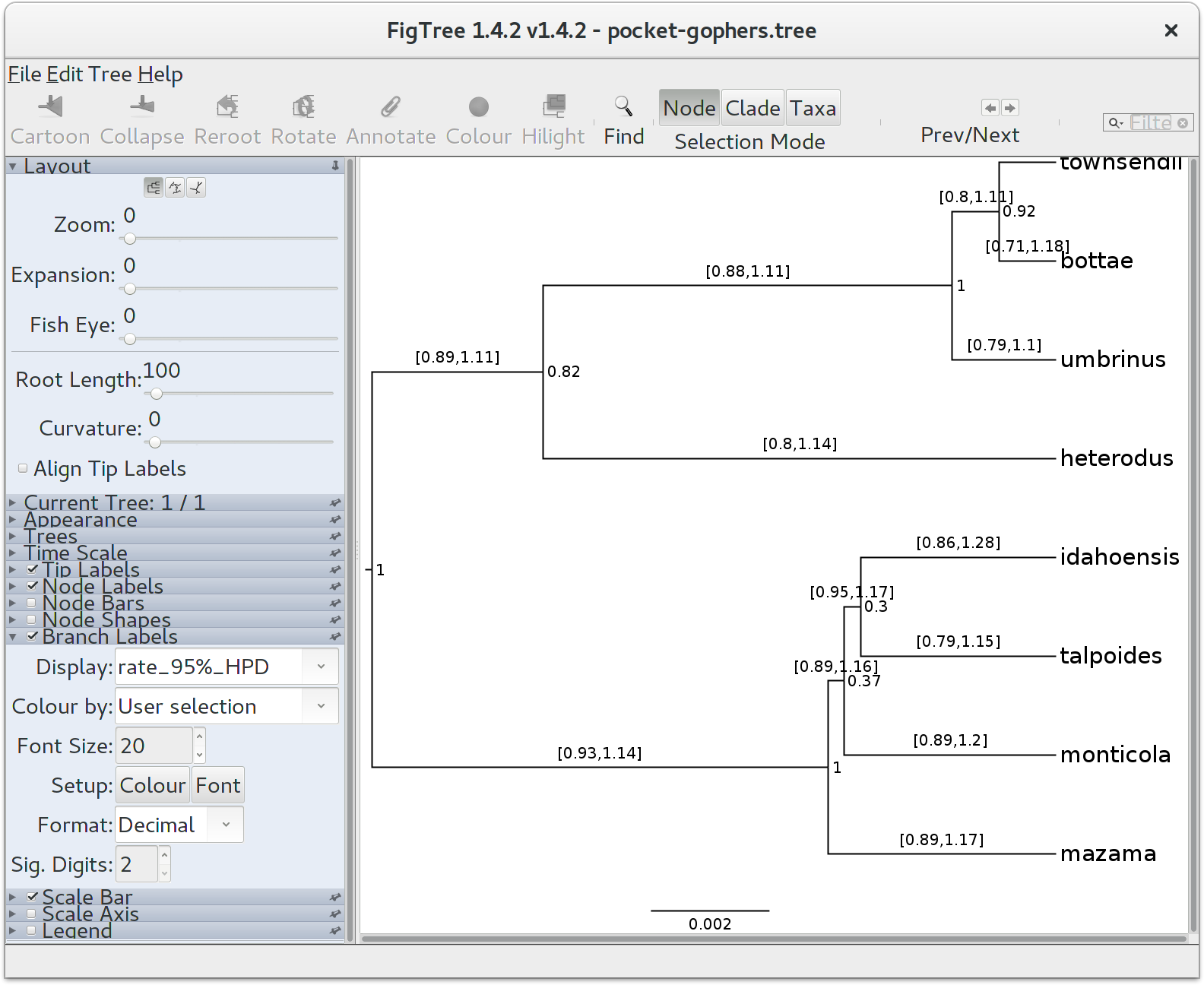
Notice that the HPD interval for per-species substitution rates all include 1.0, concordant with our previous observation that there may be no changes to the overall substitution rate along this species tree.
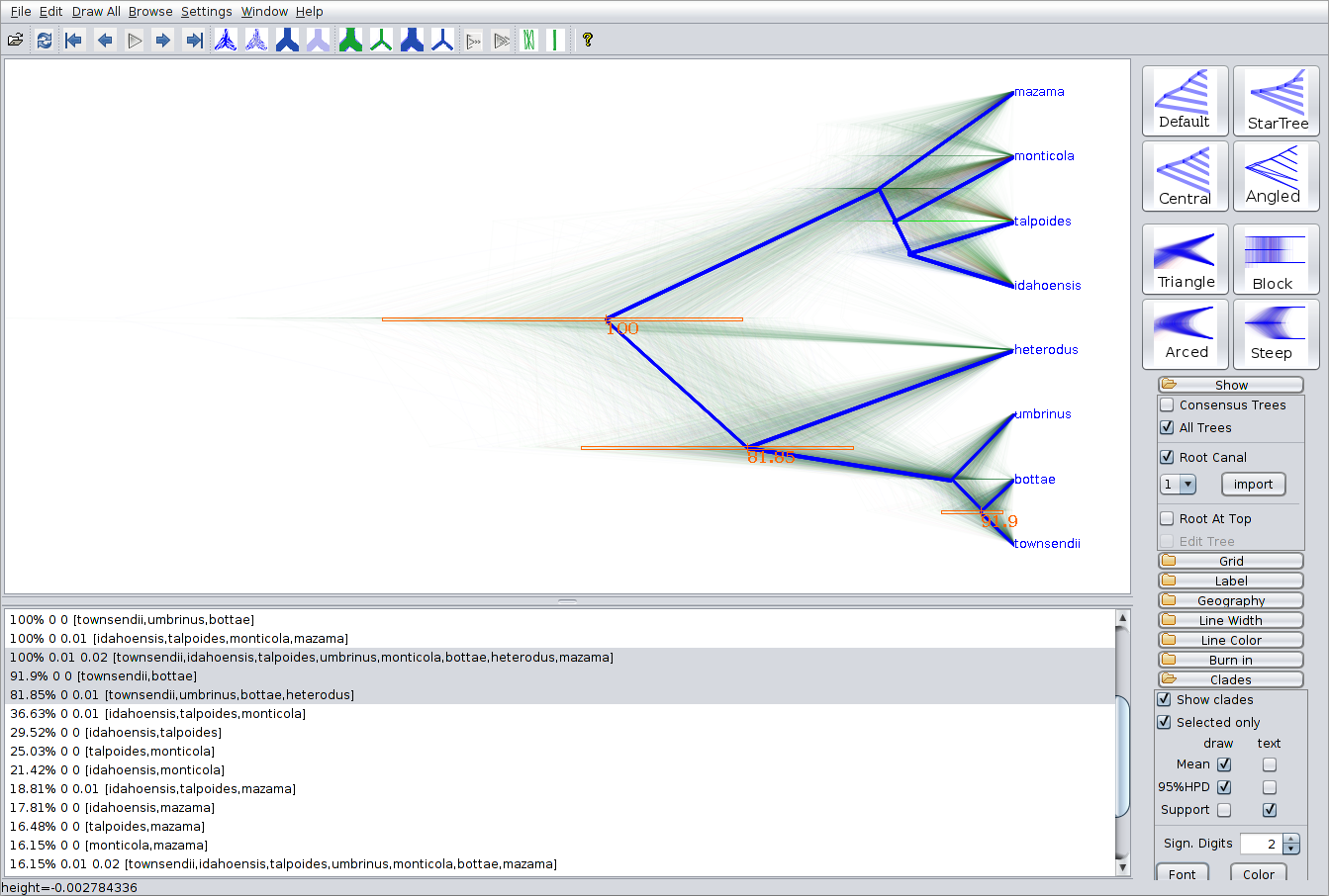
As a more Bayesian alternative to FigTree, you can load the entire species tree set into DensiTree. Open the species.trees file in DensiTree and set up the cloudogram as follows:
- Select the Central geometry from the set of options in the top-right of the main screen.
- Under Show, check the Root Canal tree to guide the eye.
- Under Clades, check Show Clades, display the means and 95\% HPDs using draw, and display the posterior support using text.
- Now, too many clades are shown, and most are not of interest. Check Selected only, then open the clade toolbar using the Window/View clade toolbar menu item. Select each clade (i.e. items with more than one species) with majority posterior support (i.e. with over 50% support) by using the shift key.
The image should look something like in the figure below. Notice that there is about 16% support for heterodus to be an outgroup, and about 82% for heterodus to be in a clade with bottea, umbinus and townsendii. Can you explain where the remaining 2% went?
Useful Links
- Bayesian Evolutionary Analysis with BEAST 2 (Drummond & Bouckaert, 2014)
- BEAST 2 website and documentation: http://www.beast2.org/
- Join the BEAST user discussion: http://groups.google.com/group/beast-users
Relevant References
- Heled, J., & Drummond, A. J. (2010). Bayesian Inference of Species Trees from Multilocus Data. Molecular Biology and Evolution, 27(3), 570–580. https://doi.org/10.1093/molbev/msp274
- Belfiore, N. M., Liu, L., & Moritz, C. (2008). Multilocus phylogenetics of a rapid radiation in the genus Thomomys (Rodentia: Geomyidae). Systematic Biology, 57(2), 294.
Citation
If you found Taming the BEAST helpful in designing your research, please cite the following paper:
Joëlle Barido-Sottani, Veronika Bošková, Louis du Plessis, Denise Kühnert, Carsten Magnus, Venelin Mitov, Nicola F. Müller, Jūlija Pečerska, David A. Rasmussen, Chi Zhang, Alexei J. Drummond, Tracy A. Heath, Oliver G. Pybus, Timothy G. Vaughan, Tanja Stadler (2018). Taming the BEAST – A community teaching material resource for BEAST 2. Systematic Biology, 67(1), 170–-174. doi: 10.1093/sysbio/syx060