


Background
Before running any phylogenetic analysis in BEAST, we need to decide on a model of molecular evolution that describes how our sequence data evolved. In particular, we need to decide on a substitution model that describes the relative rates at which different types of substitutions occur. For nucleotide data, the substitution model is typically represented as a 4x4 symmetric rate matrix with the general form:
Here, describes the rate of nucleotide change from . Due to mathematical reasons, only time reversible models are considered by BEAST. The substitution rate matrix in time reversible models takes the form:
where is the equilibrium frequency of nucleotide . The latter decomposition comes in handy to understand the parameterisation used in bModelTest, here the first matrix is referred to as rate matrix and the second is a diagonal matrix with the equilibrium frequencies on the diagonal.
The different named substitution models (e.g. JC69, HKY, TN93 and GTR) group these rates into different categories. Group here means that the rates are the same. For example, the JC69 model groups all rates together into a single rate category, i.e. . In addition, this model assumes equal equilibrium frequencies. The GTR model, however, assigns each rate to a different category and assumes a different equilibrium frequency for each nucleotide. We are therefore faced with the difficult choice of deciding a priori which one of these substitution models is most appropriate for our data.
Topic for discussion: In terms of phylogenetic inference, what would the consequences be of picking a substitution model that is overparameterized (too complex) for a given data set? What would the consequences be of picking a model that is underparameterized?
In addition to the substitution model, we also need to decide whether to include rate heterogeneity across sites. We might also want to include a proportion of invariant sites. On top of all this, we need to decide whether to estimate nucleotide base frequencies (the in the equation above) or fix them at their empirical frequencies. All of these choices leads to a bewildering number of different models to choose from. For this reason, researchers have often based their model choice on common conventions rather than on which model is most appropriate for their data.
Fortunately, nowadays we can be more sophisticated in our modeling choices and let the data inform us about which model is most appropriate using Bayesian model averaging. In this tutorial, we will use BEAST2’s model averaging tool bModelTest (Bouckaert & Drummond, 2017) to select the most appropriate substitution model for the primate mitochondrial data set we already saw in the introductory tutorial. bModelTest uses reversible jump MCMC (rjMCMC), which allows the Markov chain to jump between states representing different possible substitution models, much like we jump between different parameter states in standard Bayesian MCMC inference. This allows us to treat the substitution model as a nuisance parameter and integrate over all available (more on this later) substitution models while simultaneously estimating the phylogeny and other model parameters. Thus, parameter estimates are effectively averaged over different substitution models, weighted by the support of each model. A useful consequence is that as we are exploring the space of different substitution models we also log the proportion of time that the Markov chain spends in a particular model state. This can be interpreted as the posterior support of a model, which tells us how strongly the data and our prior beliefs support a model in comparison to other competing models.
Note that bModelTest is only able to average over a subset of substitution models that are (a) implemented in BEAST2 and (b) that it knows how to move between. Ideally we would want to integrate over all possible substitution models, but since non-reversible models are mathematically inconvenient we restrict ourselves to the set of time-reversible (symmetric) nucleotide substitution models, which leaves us with 203 possible models. In addition, we can jump between models with empirical/estimated base frequencies, with/without gamma distributed rate heterogeneity and with/without invariant sites, resulting in a total of 203 x 2 x 2 x 2 = 1,624 possible model combinations.
Programs used in this Exercise
BEAST2 - Bayesian Evolutionary Analysis Sampling Trees
BEAST2 (http://www.beast2.org) is a free software package for Bayesian evolutionary analysis of molecular sequences using MCMC and strictly oriented toward inference using rooted, time-measured phylogenetic trees. This tutorial is written for BEAST v2.7.x (Drummond & Bouckaert, 2014).
BEAUti2 - Bayesian Evolutionary Analysis Utility
BEAUti2 is a graphical user interface tool for generating BEAST2 XML configuration files.
Both BEAST2 and BEAUti2 are Java programs, which means that the exact same code runs on all platforms. For us it simply means that the interface will be the same on all platforms. The screenshots used in this tutorial are taken on a Mac OS X computer; however, both programs will have the same layout and functionality on both Windows and Linux. BEAUti2 is provided as a part of the BEAST2 package so you do not need to install it separately.
Tracer
Tracer (http://tree.bio.ed.ac.uk/software/tracer) is used to summarise the posterior estimates of the various parameters sampled by the Markov Chain. This program can be used for visual inspection and to assess convergence. It helps to quickly view median estimates and 95% highest posterior density intervals of the parameters, and calculates the effective sample sizes (ESS) of parameters. It can also be used to investigate potential parameter correlations. We will be using Tracer v1.7.0.
Practical: Selecting a substitution model
In this tutorial we will go through an analysis using bModelTest in BEAST v2.7.x and look into how to interpret the results. This tutorial assumes that you have already done some of the other tutorials and that you are familiar with the basics of using BEAUti, BEAST and Tracer.
Installing the bModelTest Package
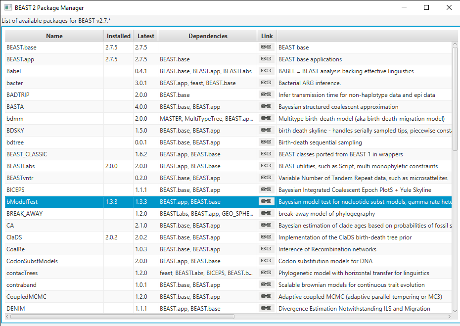
We first have to install the bModelTest (version 1.3.3 or above) package.
Open BEAUti and navigate to File > Manage Packages. Select bModelTest and then click Install/Upgrade (Figure 1). Then restart BEAUti to load the package.
The Data
We will continue analyzing the primate mitochondrial data set from the introductory tutorial.
Open BEAUti and navigate to File > Import Alignment. Select the file
primate-mtDNA.nexin the data directory.
Setting up the analysis in BEAUti
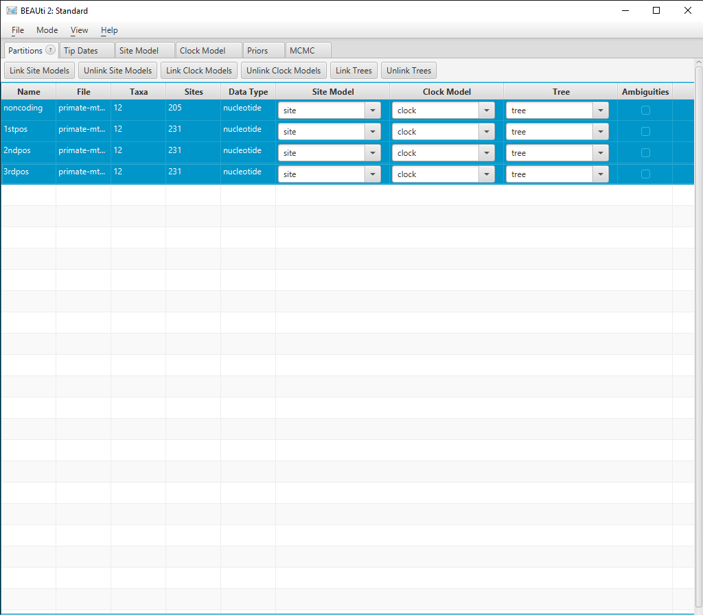
Depending on which version of the primate-mtDNA.nex file you downloaded you will find four partions (noncoding, 1stpos, 2ndpos, and 3rdpos) or five partions (coding, noncoding, 1stpos, 2ndpos, and 3rdpos). In case your file contains the coding partition (which actually consists of all 1st, 2nd, and 3rd positions), you have to delete it by selecting the respective row and clicking on the - on the bottom left. We will work with the four partions noncoding, 1stpos, 2ndpos, and 3rdpos. Additionally, we will simplify things by having all four partitions in the alignment evolve under the same Site, Clock and Tree models.
In the Partitions panel select all four partitions (with shift+click) and then click Link Site Models, Link Clock Models and Link Trees. You should rename each model something more informative than noncoding, such as site, clock and tree. Rename models by double-clicking on the drop-down boxes.
The Partition window should now look like Figure 2.
Now we want to set up our Site Model to run the model averaging analysis.
Click the Site Model tab in BEAUti and then select the drop-down box at the top which says Gamma Site Model and change it to BEAST Model Test (Figure 3).
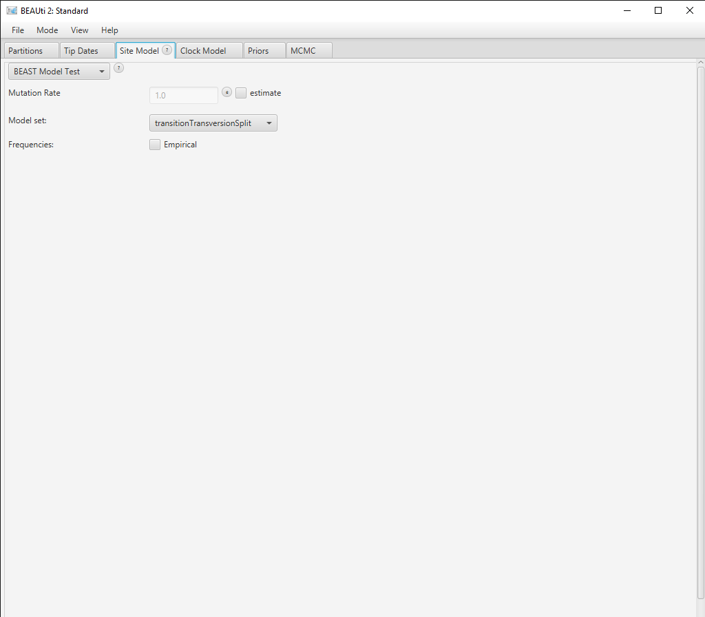
In the lower drop-down box we will keep transitionTransversionSplit selected. This tells bModelTest to only consider substitution models that differentiate between transitions (A G and C T) and transversions (all other substitutions). If all possibilities to group the rates in the substitution rate matrix, independent of whether substitutions are transitions or transersions, there are a total of 203 reversible models with symmetric rate matrices (Bouckaert & Drummond, 2017). However, if we only consider models that group transitions together with transitions but not with transversions, there are only 31 models. Selecting transitionTransversionSplit therefore dramatically reduces the number of models that we need to explore.
In the Clock Model and Prior tabs, we do not need to change any of the default settings for this tutorial.
Click the MCMC tab in BEAUti. Change the chain length to 5 000 000 and the sampling frequency to every 5 000 by changing Log Every under tracelog and treelog. This will help us to avoid autocorrelation by ensuring that we are not sampling too frequently. (You can also increase Log Every under screenlog to keep BEAST2 from producing too much screen output). Change the tracelog file name to
primate-mtDNA-bMT.logand the treelog file name toprimate-mtDNA-bMT.trees. Click File > Save As and save asprimate-mtDNA-bMT.xml. You can now close BEAUTi.
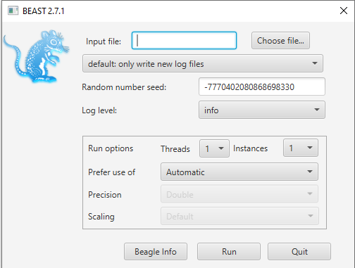
Run the analysis in BEAST
Open BEAST and choose
primate-mtDNA-bMT.xmlas the BEAST XML File (Figure 4). If BEAGLE is installed check the box to use it. Then click run.
While BEAST is running consider the following discussion points.
We did not check estimate in the box next to the Mutation Rate in the Site Model tab. Doing so makes no difference, since BEAUti constrains the mean substitution rate of all partitions to be equal to 1 (by default). Since we linked the substitution model across all partitions we effectively have only one partition, thus the substitution rate is fixed to 1.
Note that BEAUti (by default) does not allow us to estimate the clock rate in the Clock Model tab. In this analysis we only have contemporaneously sampled sequences and we did not set a calibration node as in the introductory tutorial. Thus, we have no temporal information and the clock rate is not uniquely identifiable. To make the model identifiable BEAUti arbitrarily fixes the clock rate to 1.
Topics for discussion:
Suppose we used individual substitution models for each partition. What does the estimated substitution rate for each partition represent? Would the rate of each partition be identifiable?
What would happen if we removed the constraint to have a mean substitution rate of 1? What if we also added a calibration point?
Analyzing the output in Tracer
Open the
primate-mtDNA-bMT.logfile in Tracer. There should be a long list of entries in the window on the left hand side (Figure 5).
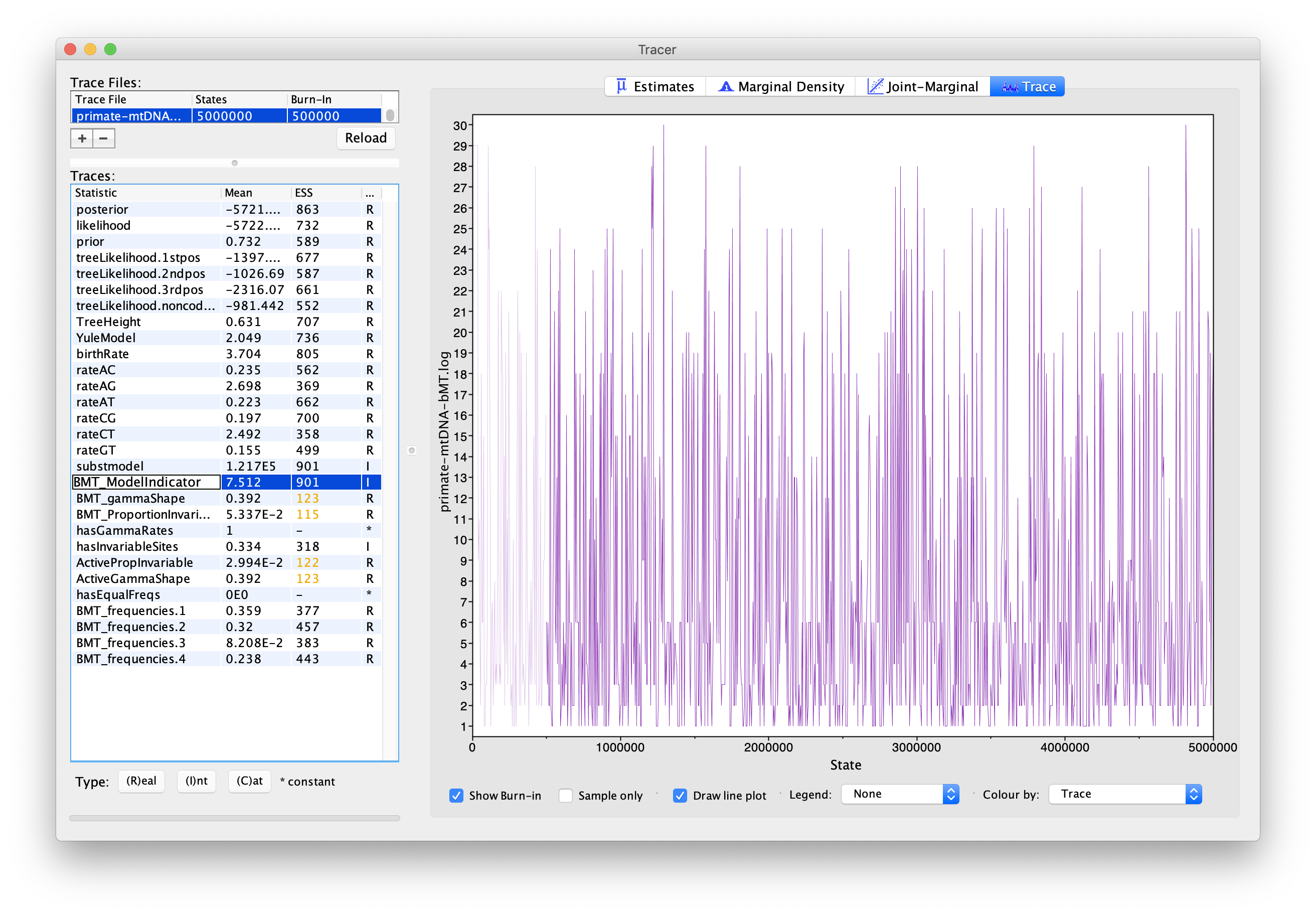
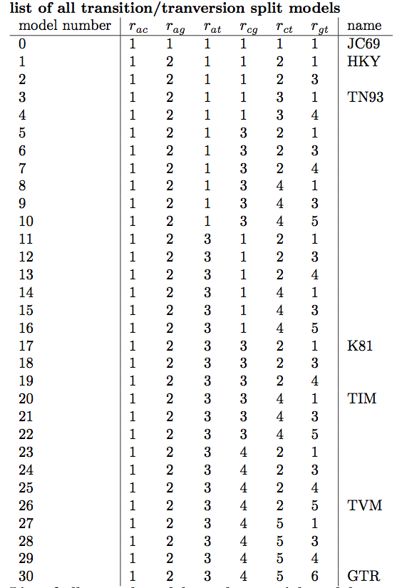
If we select BMT_ModelIndicator from the list of entries and then (I)nt for the Data type below, we can see how the Markov chain explored the space of different models by jumping between substitution models. This is best seen if we click on the Trace tab (Figure 5). Here, the sampled integer values refer to the indexes of the different substitution models. To see which index corresponds to which model, refer to (Figure 6).
Now click on the Estimates tab above. This frequency histogram shows us how much time the Markov chain spent in each model state relative to other model states, and therefore reflects the posterior support for each model. We can see that the chain spent the most time in model number 1 (Figure 7), which by consulting Figure 6 we see corresponds to the HKY model.
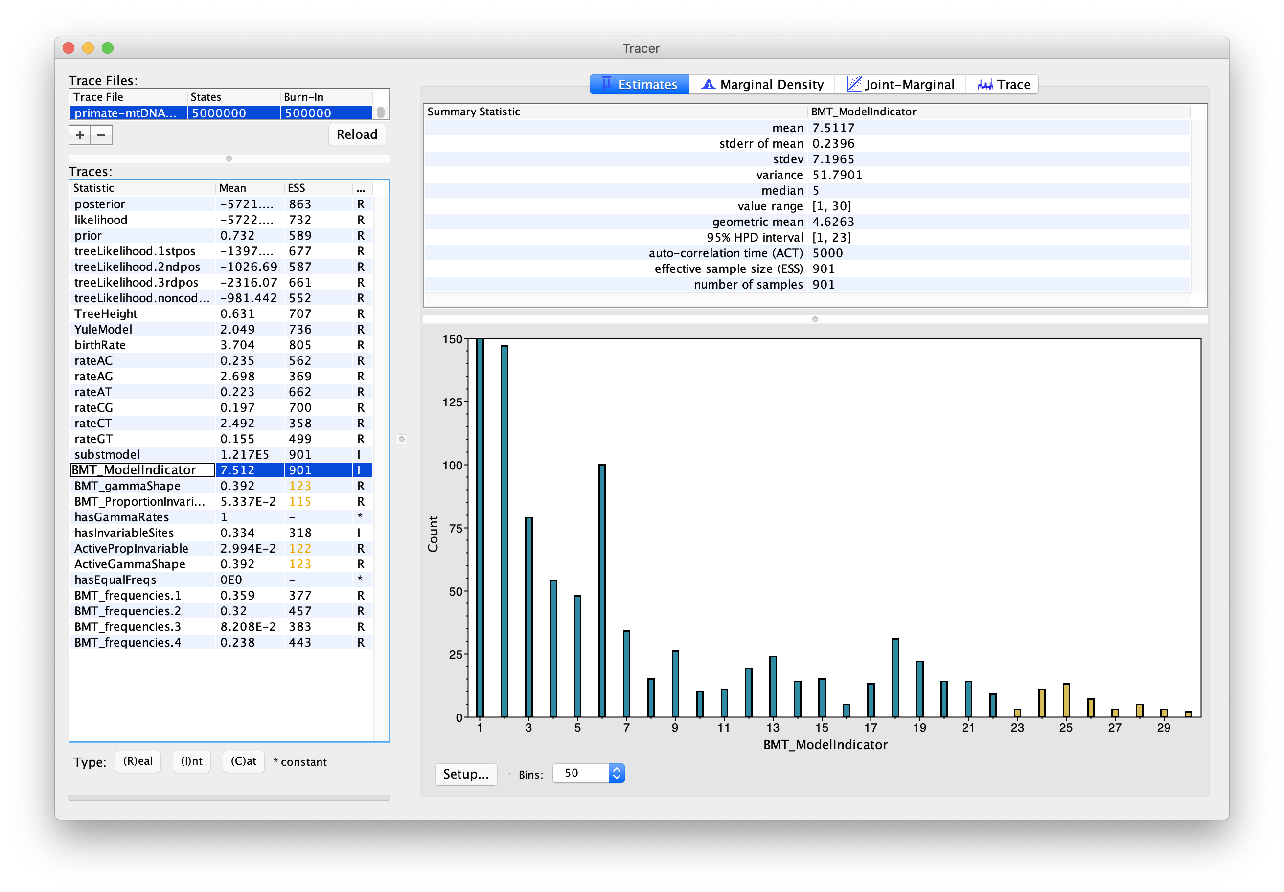
Topic for discussion: Did the chain ever visit the JC69 model? Why not?
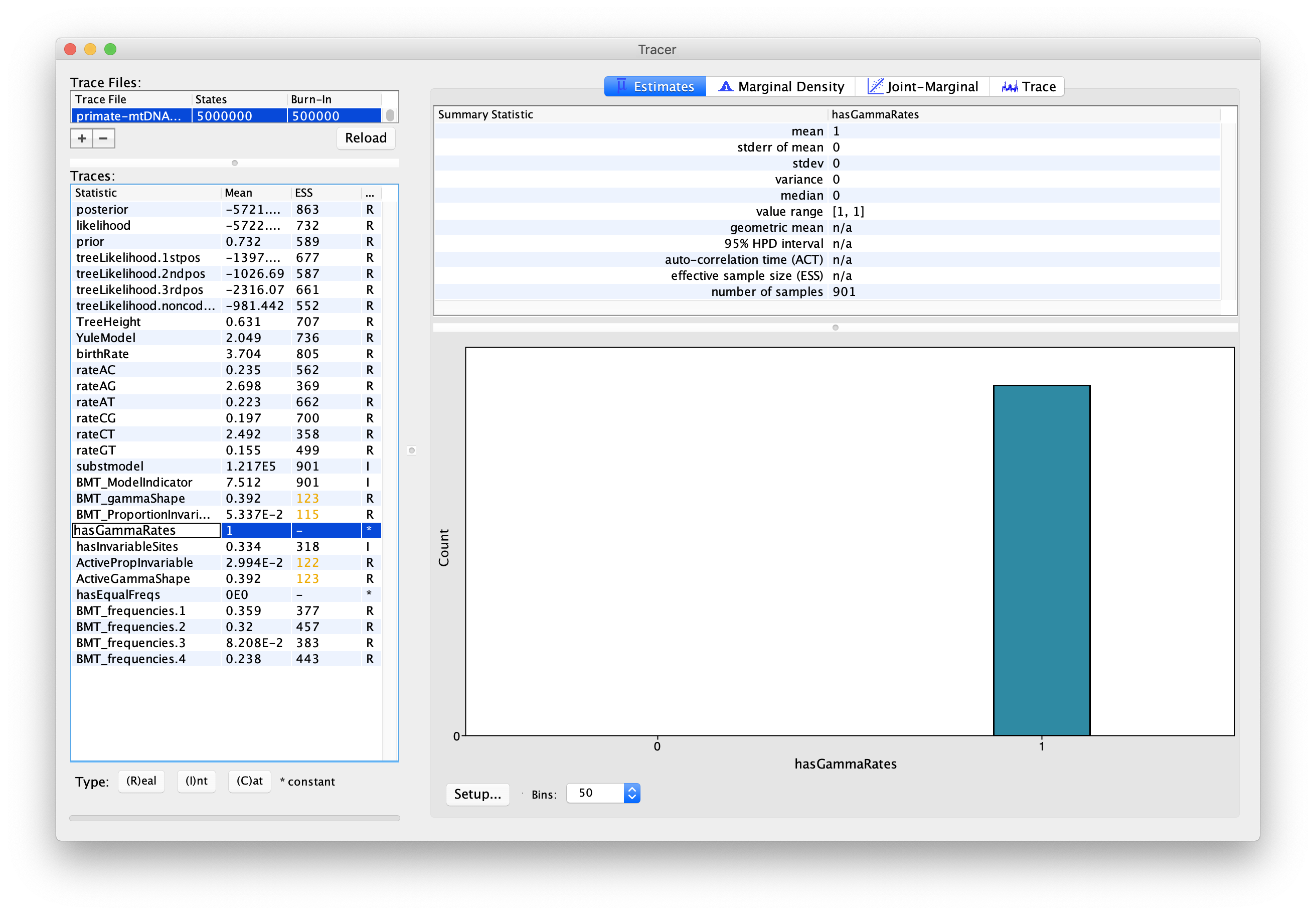
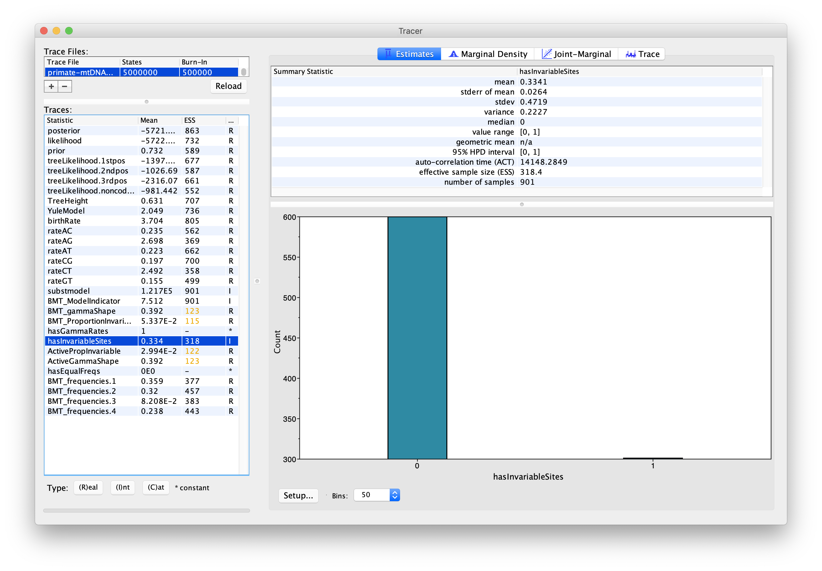
We can also use the output of our analysis to see if a model with (gamma) rate heterogeneity and/or a proportion of invariant sites is supported. If we select hasGammaRates in the window on the left and then click Estimates we see the proportion of time the chain spent in a model state with rate heterogeneity on (1) versus off (0), and thus the posterior support for a model with rate heterogeneity. Here, the chain seems to remain in a state with rate heterogeneity on, indicating very strong support for heterogeneity (Figure 8). We can also select hasInvariableSites to see if a model with invariant sites is supported. Here we see that the model spends more time in a model state with invariant sites off (0) than on (1), indicating that the presence of invariant sites are not as strongly supported (Figure 9). Note that we can also look at the traces for BMT_gammaShape and BMT_ProportionInvariant to see which values of these two parameters the chain visited.
There are a few other things we can look at in Tracer as well:
- rateAC, … ,rateGT are the substitution rates between pairs of nucleotides in the substitution matrix. Note that these rates are averaged over all the models, weighted by the time the Markov chain spent in each model state.
- ActiveGammaShape/PropInvariable are the gamma shape parameter and the proportion of variables sites when active, that is, when hasGammaRates and hasInvariableSites are selected. To get the estimate of the mean of the shape parameter, divide the mean ActiveGammaShape by the mean of hasGammaRates.
- hasEqualFreqs indicates if the chain is in a state with equal nucleotide base frequencies.
Select pairs of the rateAC, … ,rateGT parameters (using shift+click) and click on the Joint-Marginal tab to investigate parameter correlations (Figure 10). Try looking at rateAT vs. rateCG and rateCG vs rateGT).
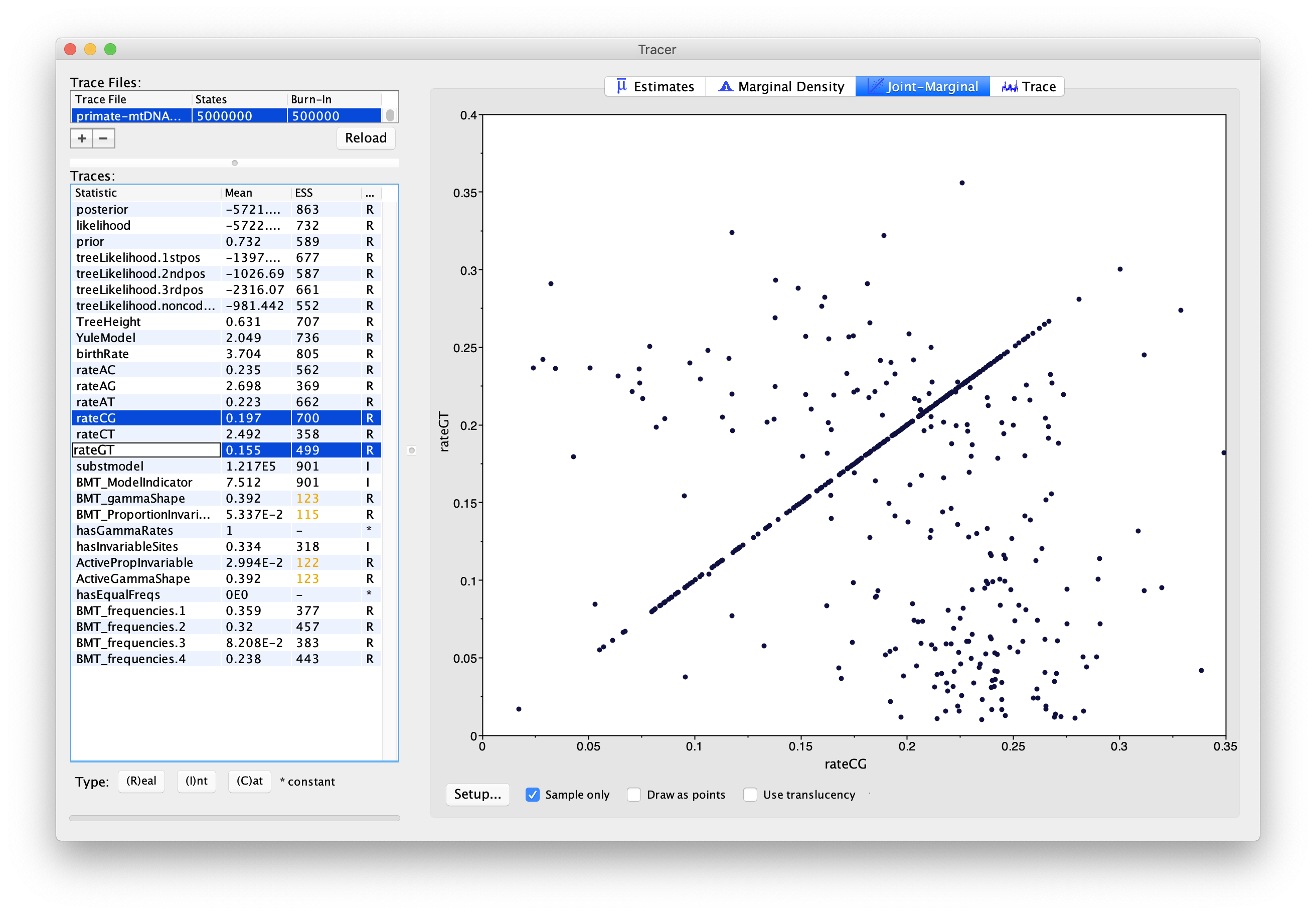
Topic for discussion: It appears that some pairs of the rate parameters are highly correlated for some samples and uncorrelated for the rest. What is happening here? Should we be worried about these parameter correlations?
Analyzing the output using BModelAnalyzer
Another really nice feature of bModelTest is that we can graphically analyze the output using the BModelAnalyser App.
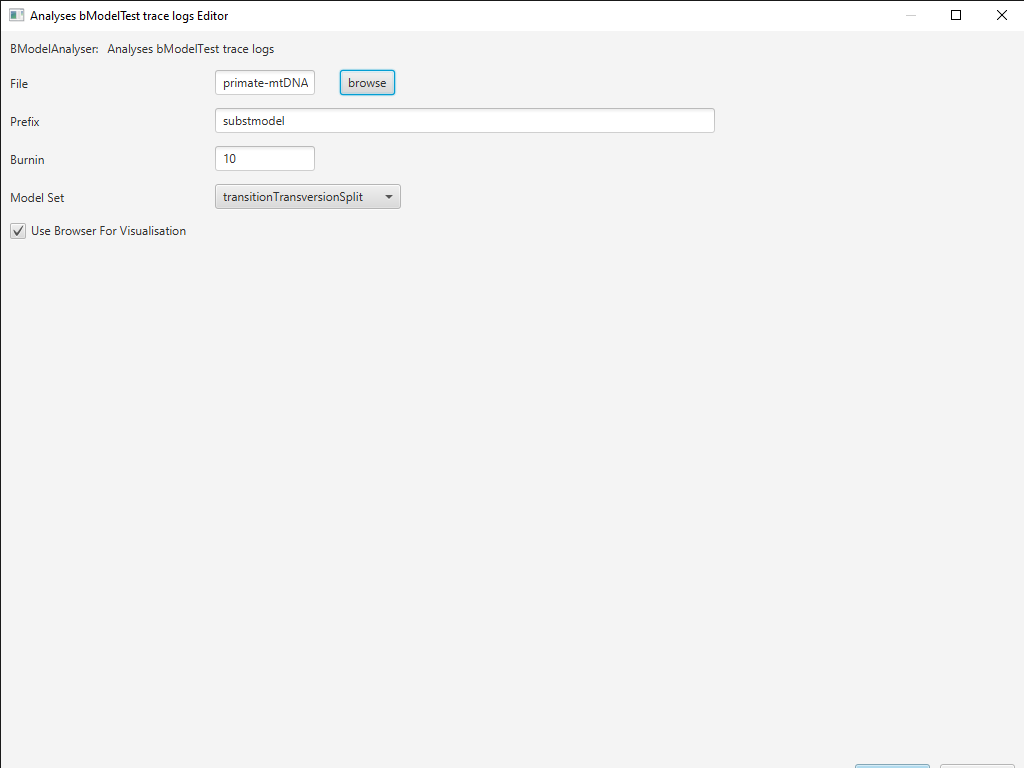
In BEAUti, select File > Launch Apps. You can filter the apps by the package they are attached to, here bModelTest (Figure 11). Find and launch the BModelAnalyser App. A dialogue window should pop up (Figure 12). Enter
primate-mtDNA-bMT.logas the file to analyze. You can leave the other entries at their default settings but make sure transitionTransversionSplit is selected for the Model Set and the box next to Use Browser For Visualization is checked. Then click OK.

After BModelAnalyser runs, a new window should appear in your default web browser that represents the model selection results graphically (Figure 13). This graph depicts the nested relationship of the different substitution models: an arrow pointing from one model to another indicates that the model at the tail is nested within the model at the head of the arrow. As we can see, JC69 is nested within all other models and all other models are nested within GTR.
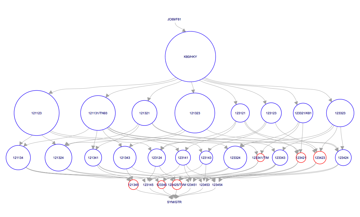
The area of the circle surrounding each model is proportional to the the posterior support for that model. The colours represent whether the model is contained within the 95% credible set (blue) or not (red). For the primate data set, the HKY model clearly has the highest posterior support (Figure 13). However, other models such as TN93 and two unnamed models, 121323 and 121123, also have fairly high posterior support. The six digit model code describes how the different substitution rates are grouped in the order of , , , , and . For instance, 121323 is a slight variant of the HKY model with an additional group for the rates and . The six digit codes for all models are shown in Figure 6.
Topic for discussion: We have used bModelTest to explore a large set of substitution models. But how do we know that any of the substitution models actually fit the observed sequence data well?
Acknowledgment
This tutorial is based on the original bModelTest tutorial by Remco Bouckaert.
Useful Links
- Official bModelTest documentation: https://github.com/BEAST2-Dev/bModelTest/wiki
- The original bModelTest tutorial is available here: https://github.com/BEAST2-Dev/bModelTest/releases/download/v0.3.0/bModelTestTutorial.pdf and is also included in the source code.
Relevant References
- Bouckaert, R. R., & Drummond, A. J. (2017). bModelTest: Bayesian phylogenetic site model averaging and model comparison. BMC Evolutionary Biology, 17(1), 42. https://doi.org/10.1186/s12862-017-0890-6
- Drummond, A. J., & Bouckaert, R. R. (2014). Bayesian evolutionary analysis with BEAST 2. Cambridge University Press.
Citation
If you found Taming the BEAST helpful in designing your research, please cite the following paper:
Joëlle Barido-Sottani, Veronika Bošková, Louis du Plessis, Denise Kühnert, Carsten Magnus, Venelin Mitov, Nicola F. Müller, Jūlija Pečerska, David A. Rasmussen, Chi Zhang, Alexei J. Drummond, Tracy A. Heath, Oliver G. Pybus, Timothy G. Vaughan, Tanja Stadler (2018). Taming the BEAST – A community teaching material resource for BEAST 2. Systematic Biology, 67(1), 170–-174. doi: 10.1093/sysbio/syx060