


Background
Phylogeographic methods can help reveal the movement of genes between populations of organisms. This has been widely used to quantify pathogen movement between different host populations, the migration history of humans, and the geographic spread of languages or the gene flow between species using the location or state of samples alongside sequence data. Phylogenies therefore offer insights into migration processes not available from classic epidemiological or occurrence data alone.
The structured coalescent allows to coherently model the migration and coalescent process, but struggles with complex datasets due to the need to infer ancestral migration histories. Thus, approximations to the structured coalescent, which integrate over all ancestral migration histories, have been developed. This tutorial gives an introduction into how a MASCOT analysis in BEAST2 can be set-up. MASCOT is short for Marginal Approximation of the Structured COalescen T (Müller et al., 2018) and implements a structured coalescent approximation (Müller et al., 2017). This approximation doesn’t require migration histories to be sampled using MCMC and therefore allows to analyse phylogenies with more than three or four states.
Programs used in this Exercise
BEAST2 - Bayesian Evolutionary Analysis Sampling Trees 2
BEAST2 (http://www.beast2.org) is a free software package for Bayesian evolutionary analysis of molecular sequences using MCMC and strictly oriented toward inference using rooted, time-measured phylogenetic trees. This tutorial is written for BEAST v2.7.x (Drummond & Bouckaert, 2014).
BEAUti2 - Bayesian Evolutionary Analysis Utility
BEAUti2 is a graphical user interface tool for generating BEAST2 XML configuration files.
Both BEAST2 and BEAUti2 are Java programs, which means that the exact same code runs on all platforms. For us it simply means that the interface will be the same on all platforms. The screenshots used in this tutorial are taken on a Mac OS X computer; however, both programs will have the same layout and functionality on both Windows and Linux. BEAUti2 is provided as a part of the BEAST2 package so you do not need to install it separately.
TreeAnnotator
TreeAnnotator is used to summarise the posterior sample of trees to produce a maximum clade credibility tree. It can also be used to summarise and visualise the posterior estimates of other tree parameters (e.g. node height).
TreeAnnotator is provided as a part of the BEAST2 package so you do not need to install it separately.
Tracer
Tracer (http://tree.bio.ed.ac.uk/software/tracer) is used to summarise the posterior estimates of the various parameters sampled by the Markov Chain. This program can be used for visual inspection and to assess convergence. It helps to quickly view median estimates and 95% highest posterior density intervals of the parameters, and calculates the effective sample sizes (ESS) of parameters. It can also be used to investigate potential parameter correlations. We will be using Tracer v1.7.2.
FigTree
FigTree (http://tree.bio.ed.ac.uk/software/figtree) is a program for viewing trees and producing publication-quality figures. It can interpret the node-annotations created on the summary trees by TreeAnnotator, allowing the user to display node-based statistics (e.g. posterior probabilities). We will be using FigTree v1.4.4.
Practical: Parameter and State inference using the approximate structured coalescent
In this tutorial we will estimate migration rates, effective population sizes and locations of internal nodes using the marginal approximation of the structured coalescent implemented in BEAST2, MASCOT (Müller et al., 2018).
The aim is to:
- Learn how to infer structure from trees with sampling location
- Get to know how to choose the set-up of such an analysis
- Learn how to read the output of a MASCOT analysis
Setting up an analysis in BEAUti
Download MASCOT
First, we have to download the package MASCOT using the BEAUTi package manager. Go to File » Manage Packages and download the package MASCOT.
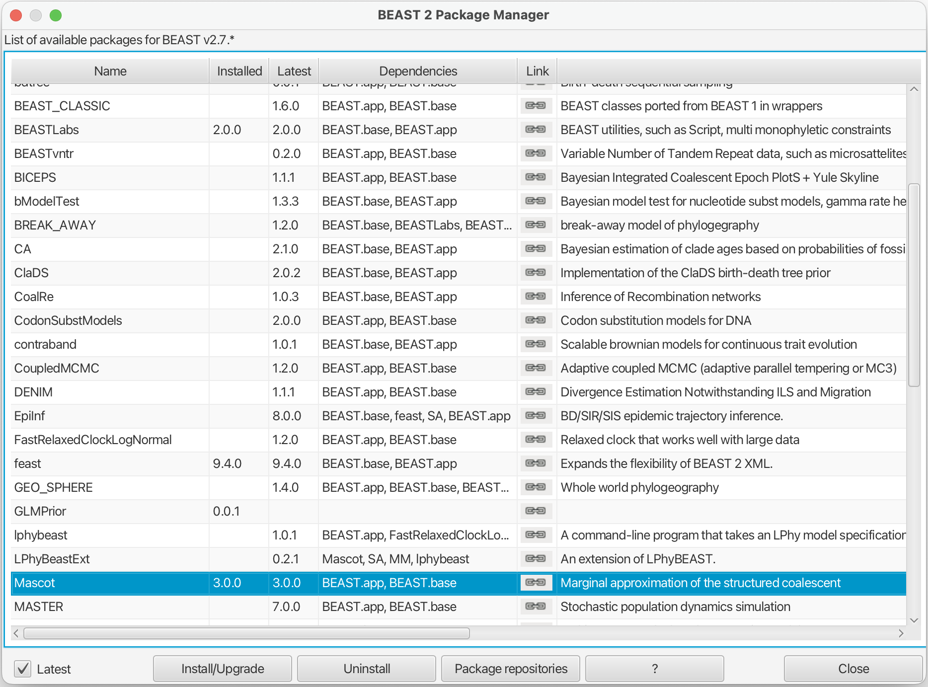
MASCOT will only be available in BEAUti once you close and restart the program.
Loading the Influenza A/H3N2 Sequences (Partitions)
The sequence alignment is in the file H3N2.nexus. Right-click on this link and save it to a folder on your computer. Once downloaded, this file can either be drag-and-dropped into BEAUti or added by using BEAUti’s menu system via File » Import Alignment. Once the sequences are added, we need to specify the sampling dates.
Get the sampling times (Tip Dates)
Open the “Tip Dates” panel and then select the “Use tip dates” checkbox.
The sampling times are encoded in the sequence names. We can tell BEAUti to use these by clicking the Auto-configure button. The sampling times appear following the third vertical bar “|” in the sequence name. To extract these times, select “split on character”, enter “|” (without the quotes) in the text box immediately to the right, and then select “3” from the drop-down box to the right, as shown in the figure below.
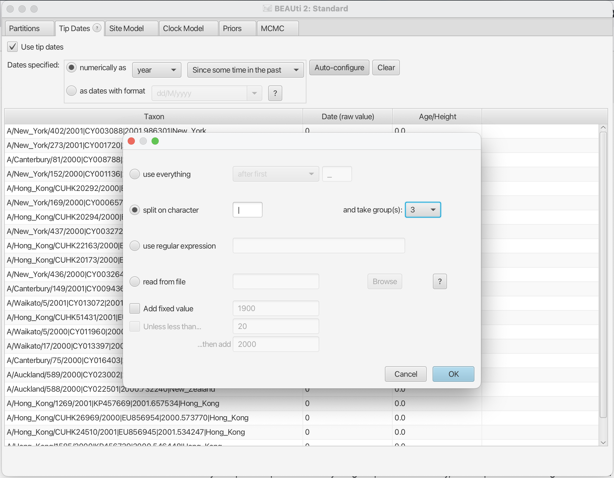
Clicking “Ok” should now populate the table with the sample times extracted from the sequence names: the column Date should now have values between 2000 and 2002 and the column Height should have values from 0 to 2. The heights denote the time difference from a sequence to the most recently sampled sequence. If everything is specified correctly, the sequence with Height 0.0 should have Date 2001.9.
Specify the Site Model (Site Model)
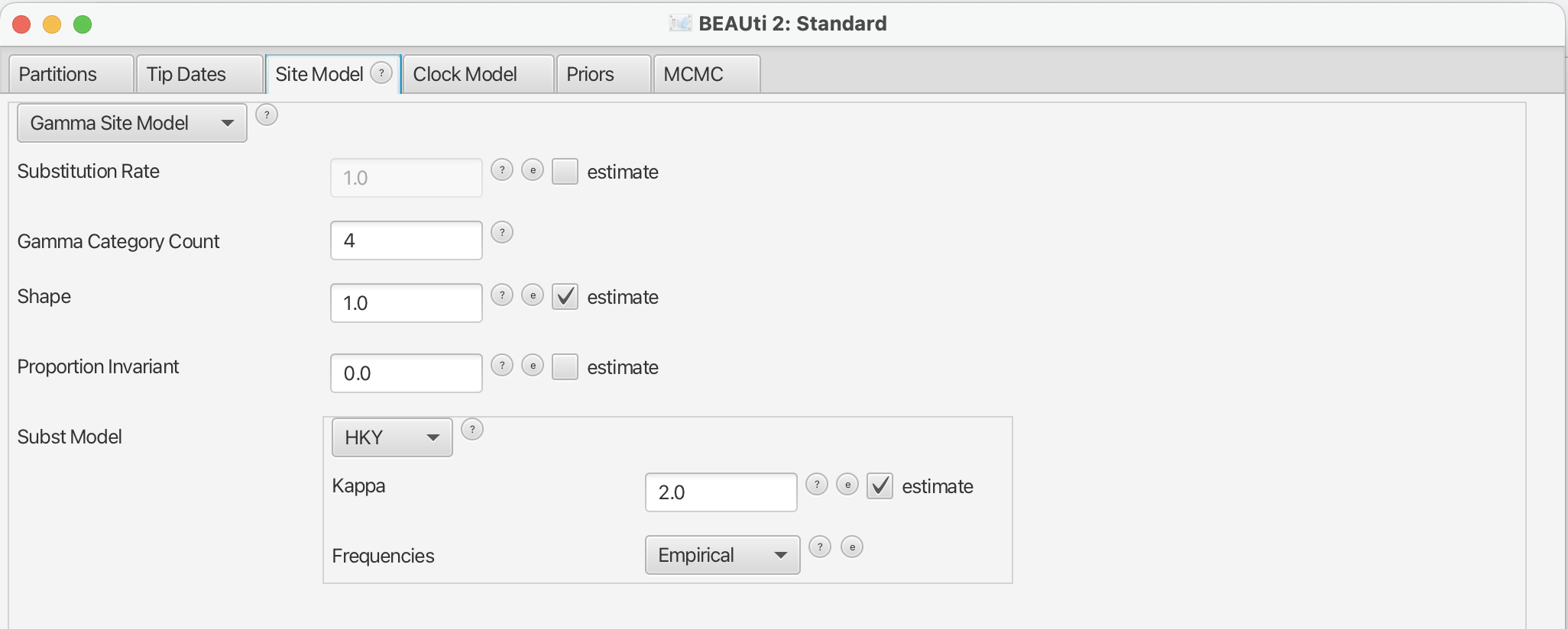
Next, we have to specify the site model. To do this, choose the “Site Model” tab. For Influenza Hemagluttanin sequences as we have here, HKY is the most commonly used model of nucleotide evolution. This model allows for differences in transversion and transition rates, meaning that changes between bases that are chemically more closely related (transitions) are allowed to have a different rate to changes between bases that chemically more distinct (transversions). Additionally, we should allow for different rate categories for different sites in the alignment. This can be done by setting the Gamma Category Count to 4, which is just a value that has typically been used. Make sure that estimate is checked next to the shape parameter. To reduce the number of parameters we have to estimate, we can set Frequencies to Empirical.
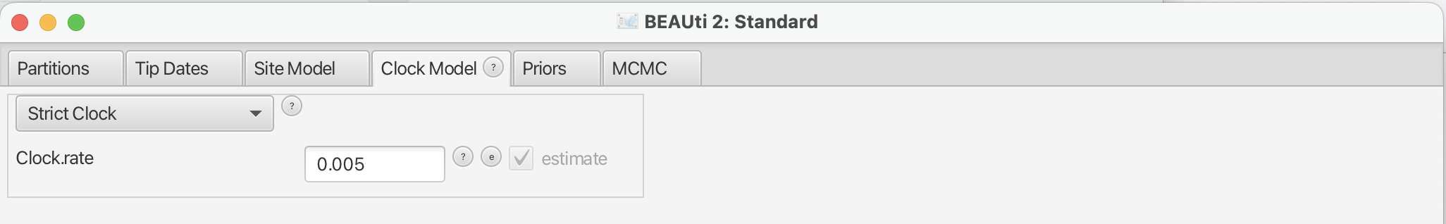
Set the clock model (Clock Model)
For rapidly evolving viruses, the assumption of a strict molecular clock is often made, meaning that the molecular clock is the same on each branch of the phylogeny. To decrease the burnin phase, we can set the initial value to 0.005.
Get the sampling locations (Tip Locations)
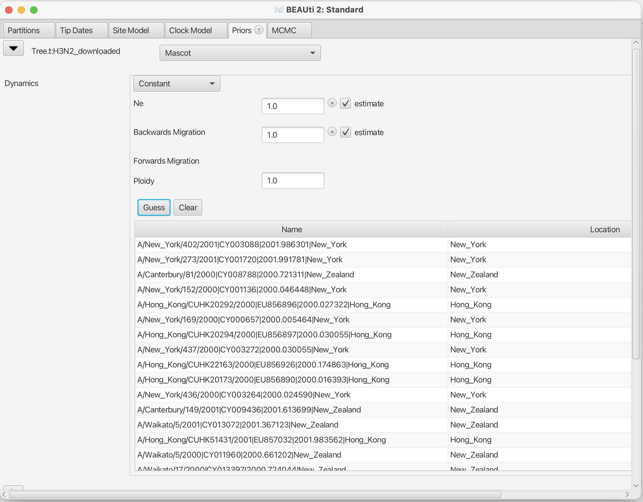
We first have to choose the tree prior, which in this case is MASCOT. We do this by switching to the “Priors” tab. Search the drop down menu next to Tree.t:H3N2 and choose MASCOT.
By default, the rate dynamics for this setting is Constant, which means that effective population sizes and migration rates are assumed to be constant through time.
We next have to define the sampling location of the individual tips.
Initially the column Location should be NOT_SET for every sequence. After clicking the Guess button, you can split the sequence on the vertical bar “|” again by selecting “split on character” and entering “|” in the box. However, the locations are in the fourth group, so this time choose “4” from the drop-down menu. After clicking the OK button, the window should look like the one shown in the figure below:
Specify the priors (Priors)
Now, we need to set the priors for the various parameters of the model. You can find the parameter priors below the tree prior.
First, consider the effective population size parameter Ne. Since we have only a few samples per location, meaning little information about the different effective population sizes, we will need an informative prior. In this case we will use a log normal prior with parameters M=0 and S=1. (These are respectively the mean and variance of the corresponding normal distribution in log space.) To use this prior, choose “Log Normal” from the drop down menu to the right of the Ne.t:H3N2 parameter label, then click the arrow to the left of the same label and fill in the parameter values appropriately (i.e. M=0 and S=1). Ensure that the “Mean In Real Space” checkbox remains unchecked.
The existing exponential distribution as a prior on the migration rate puts much weight on lower values while not prohibiting larger ones. For migration rates, a prior that prohibits too large values while not greatly distinguishing between very small and very very small values is generally a good choice. Be aware however that the exponential distribution is quite an informative prior: one should be careful that to choose a mean so that feasible rates are at least within the 95% HPD interval of the prior. (This can be determined by clicking the arrow to the left of the parameter name and looking at the values below the graph that appears on the right.) We keep the default mean value of 1.
Finally, set the prior for the clock rate. We have a good idea about the clock rate of Influenza A/H3N2 Hemagglutinin. From previous work by other people, we know that the clock rate will be around 0.005 substitution per site per year. To include that prior knowledge, we can set the prior on the clock rate to a Log Normal distribution with mean in real space set to 0.005. To specify the mean in real space, make sure that the box “Mean In Real Space” is checked. If we set the S value to 0.25, we say that we expect the clock rate to be with 95% certainty between 0.00321 and 0.00731.
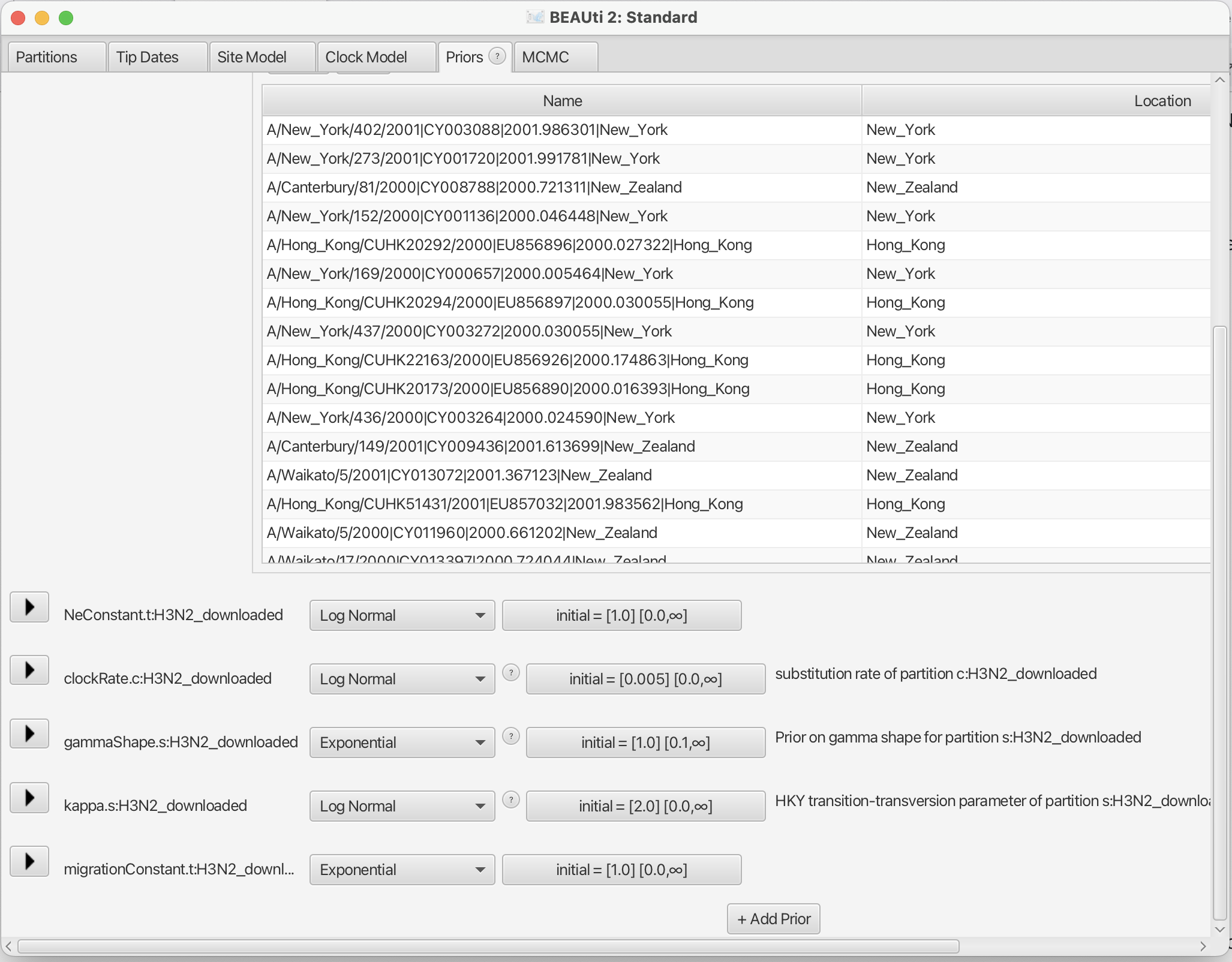
We keep the default priors for the parameters gammaShape and kappa.
Specify the MCMC chain length (MCMC)
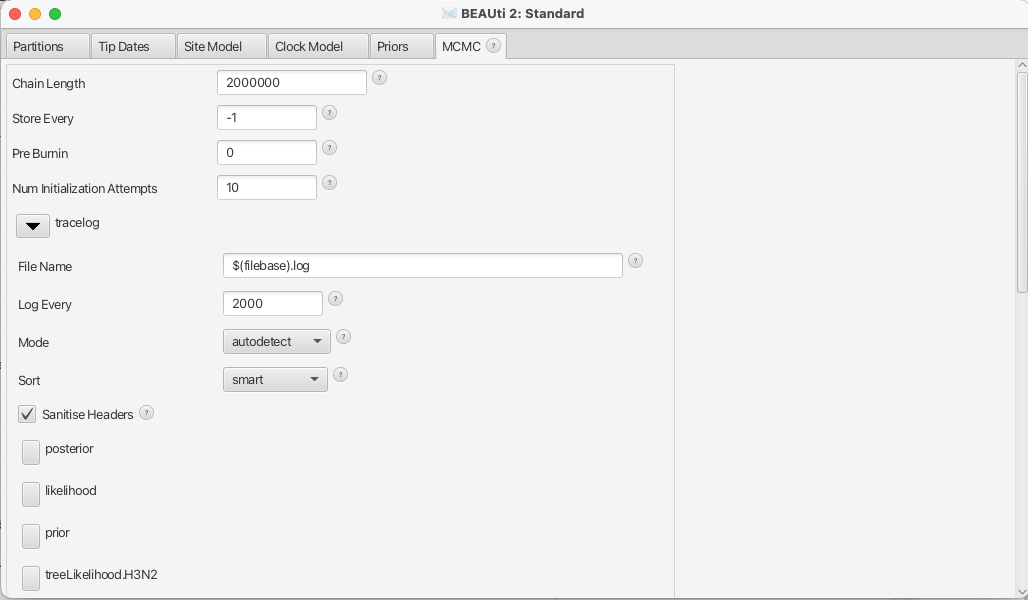
Now switch to the “MCMC” tab. Here we can set the length of the MCMC
chain and decide how frequently the parameter and trees are
logged. For this dataset, 2 million iterations should be
sufficient. In order to have enough samples but not create too large
files, we can set the logEvery to 2000, so we have 1001 samples
overall. Do this for the tracelog and the treelog.
Next, we have to save the *.xml file using File » Save
as.
Run the Analysis using BEAST2
Run the *.xml using BEAST2 or use finished runs from the precooked-runs folder. The analysis should take about 6 to 7 minutes. If you want to learn some more about what the migration rates we actually estimate, have a look at this blog post of Peter Beerli http://popgen.sc.fsu.edu/Migrate/Blog/Entries/2013/3/22_forward-backward_migration_rates.html.
Analyse the log file using Tracer
First, we can open the *.log file in tracer to check if the MCMC has converged. The ESS value should be above 200 for almost all values and especially for the posterior estimates.
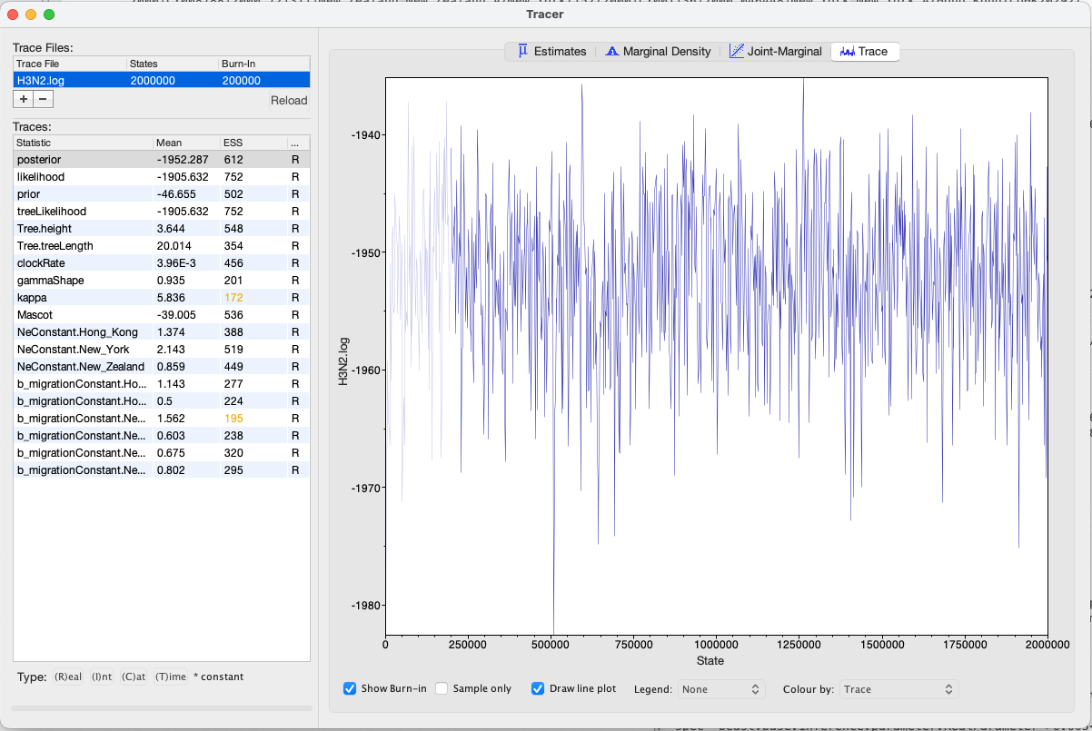
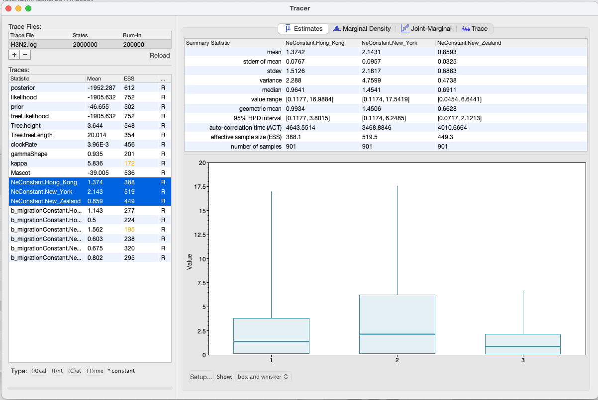
We can have a look at the marginal posterior distributions for the effective population sizes. New York is inferred to have the largest effective population size before Hong Kong and New Zealand. This tells us that two lineages that are in New Zealand are expected to coalesce quicker than two lineages in Hong Kong or New York.
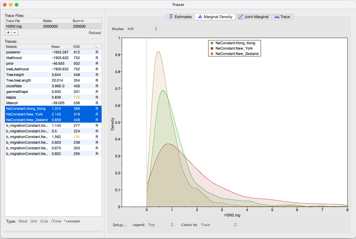
In this example, we have relatively little information about the effective population sizes of each location. This can lead to estimates that are greatly informed by the prior. Additionally, there can be great differences between median and mean estimates. The median estimates are generally more reliable since they are less influence by extreme values.
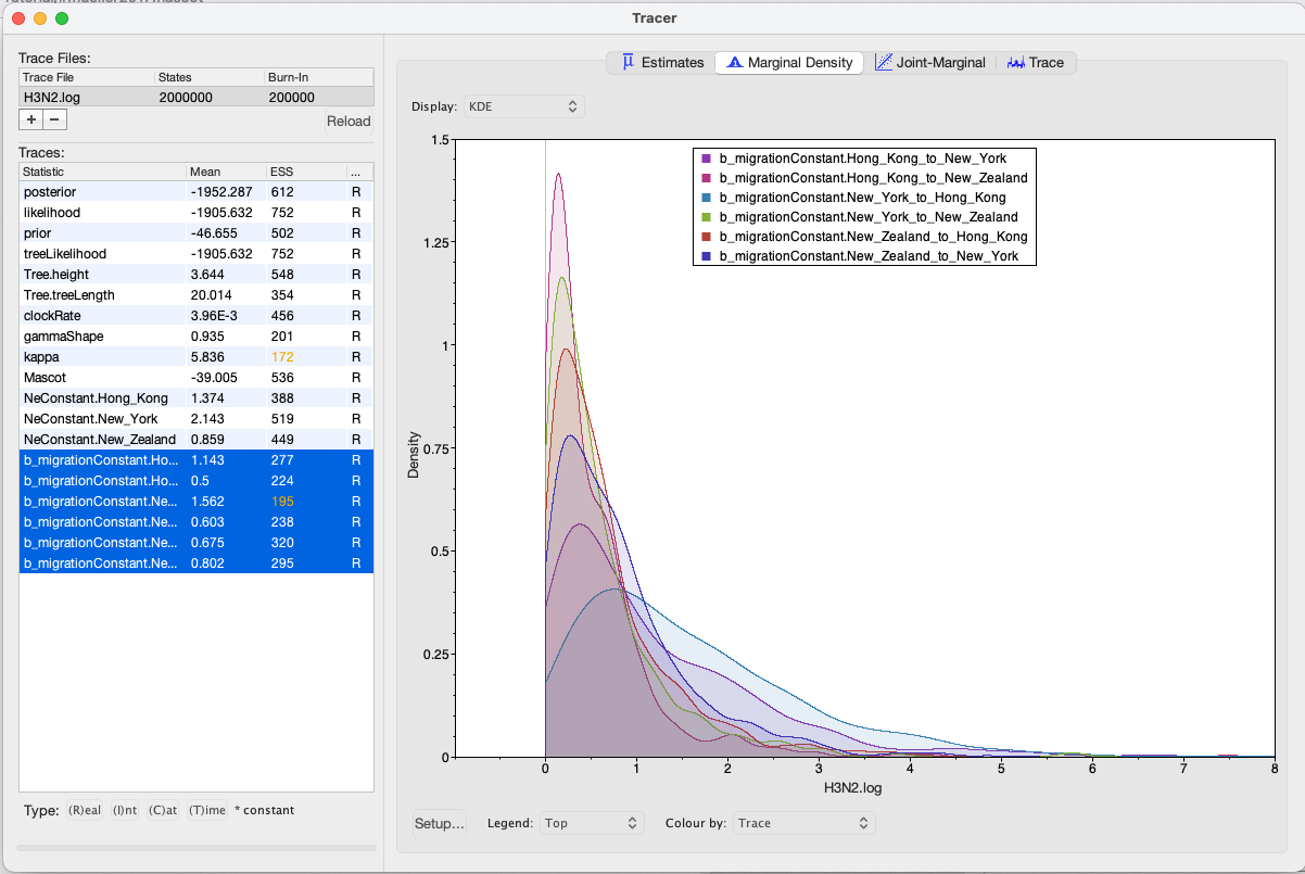
We can then look at the inferred migration rates. The migration rates have the label b_migration.*, meaning that they are backwards in time migration rates. The highest rates are from New York to Hong Kong. Because they are backwards in time migration rates, this means that lineages from New York are inferred to be likely from Hong Kong if we’re going backwards in time. In the inferred phylogenies, we should therefore make the observation that lineages ancestral to samples from New York are inferred to be from Hong Kong backwards.
A more in depth explanation of what backwards migration really are can be found here http://popgen.sc.fsu.edu/Migrate/Blog/Entries/2013/3/22_forward-backward_migration_rates.html
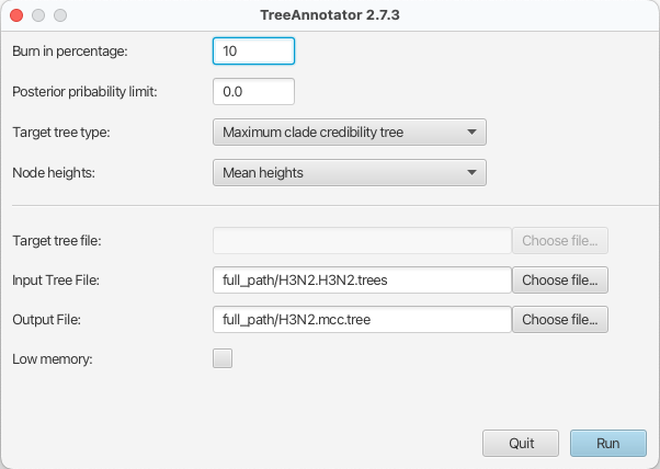
Make the MCC tree using TreeAnnotator
Next, we want to summarize the trees. This we can do using TreeAnnotator. Open the program and then set the options as below. You have to specify the Burnin percentage, the Node heights, Input Tree File and the Output File. Use the typed trees in the file H3N2.H32.trees as Input Tree File. After clicking Run the program should summarize the trees.
Check the MCC tree using FigTree
In each logging step of the tree during the MCMC, MASCOT logs several different things. It logs the inferred probability of each node being in any possible location. In this example, these would be the inferred probabilities of being in Hong Kong, New York and New Zealand. Additonally, it logs the most likely location of each node.
After opening the MCC tree in FigTree, we can visualize several things. To color branches, you can go to Appearance » Colour by and select max. This is the location that was inferred to be most often the most likely location of the node.
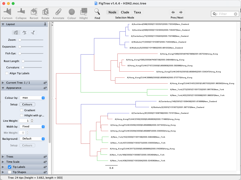
We can now determine if lineages ancestral to samples from New York are actually inferred to be from Hong Kong, or the probability of the root being in any of the locations.
To get the actual inferred probabilities of each node being in any of the 3 locations, you can go to Node Labels » Display an then choose Hong_Kong, New_York or New_Zealand. These are the actual inferred probabilities of the nodes being in any location.
It should however be mentioned that the inference of nodes being in a particular location makes some simplifying assumptions, such as that there are no other locations (i.e. apart from the sampled locations) where lineages could have been.
Another important thing to know is that currently, we assume rates to be constant. This means that we assume that the population size of the different locations does not change over time. We also make the same assumption about the migration rates through time.
Errors that can occur (Work in progress)
One of the errors message that can occur regularly is the following:
too many iterations, return negative infinity
This occurs when the integration step size of the ODE’s to compute the probability of observing a phylogenetic tree in MASCOT is becoming too small.
This generally occurs if at least one migration rate is really large or at least one effective population size is really small (i.e. the coalescent rate is really high).
This causes integration steps to be extremely small, which in turn would require a lot of time to compute the probability of a phylogenetic tree under MASCOT.
Instead of doing that, this state is rejected by assigning its log probability the value negative infinity.
This error can have different origins and a likely incomplete list is the following:
- The priors on migration rates put too much weight on really high rates. To fix this, reconsider your priors on the migration rates. Particularly, check if the prior on the migration rates make sense in comparison to the height of the tree. If, for example, the tree has a height of 1000 years, but the prior on the migration rate is exponential with mean 1, then the prior assumption is that between any two states, we expected approximately 1000 migration events.
- The prior on the effective population sizes is too low, meaning that the prior on the coalescent rates (1 over the effective population size) is too high. This can for example occur when the prior on the effective population size was chosen to be 1/X. To fix, reconsider your prior on the effective population size.
- There is substantial changes of the effective population sizes and/or migration rates over time that are not modeled. In that case, changes in the effective population sizes or migration rates have to be explained by population structure, which can again lead to some effective population sizes being very low and some migration rates being very high. In that case, there is unfortunately not much that can be done, since MASCOT is not an appropriate model for the dataset.
- There is strong subpopulation structure within the different subpopulations used. In that case, reconsider if the individual sub-populations used are reasonable.
Useful Links
If you interested in the derivations of the marginal approximation of the structured coalescent, you can find them here (Müller et al., 2017). This paper also explains the mathematical differences to other methods such as the theory underlying BASTA. To get a better idea of how the states of internal nodes are calculated, have a look in this paper (Müller et al., 2018).
- MASCOT source code: https://github.com/nicfel/Mascot
- Bayesian Evolutionary Analysis with BEAST 2 (Drummond & Bouckaert, 2014)
- BEAST 2 website and documentation: http://www.beast2.org/
- Join the BEAST user discussion: http://groups.google.com/group/beast-users
Relevant References
- Müller, N. F., Rasmussen, D., & Stadler, T. (2018). MASCOT: Parameter and state inference under the marginal structured coalescent approximation. Bioinformatics, bty406. https://doi.org/10.1093/bioinformatics/bty406
- Müller, N. F., Rasmussen, D. A., & Stadler, T. (2017). The Structured Coalescent and its Approximations. Molecular Biology and Evolution, msx186.
- Drummond, A. J., & Bouckaert, R. R. (2014). Bayesian evolutionary analysis with BEAST 2. Cambridge University Press.
Citation
If you found Taming the BEAST helpful in designing your research, please cite the following paper:
Joëlle Barido-Sottani, Veronika Bošková, Louis du Plessis, Denise Kühnert, Carsten Magnus, Venelin Mitov, Nicola F. Müller, Jūlija Pečerska, David A. Rasmussen, Chi Zhang, Alexei J. Drummond, Tracy A. Heath, Oliver G. Pybus, Timothy G. Vaughan, Tanja Stadler (2018). Taming the BEAST – A community teaching material resource for BEAST 2. Systematic Biology, 67(1), 170–-174. doi: 10.1093/sysbio/syx060